Xarray Fundamentals
Contents
Xarray Fundamentals#
Xarray data structures#
Like Pandas, xarray has two fundamental data structures:
a
DataArray, which holds a single multi-dimensional variable and its coordinatesa
Dataset, which holds multiple variables that potentially share the same coordinates
DataArray#
A DataArray has four essential attributes:
values: anumpy.ndarrayholding the array’s valuesdims: dimension names for each axis (e.g.,('x', 'y', 'z'))coords: a dict-like container of arrays (coordinates) that label each point (e.g., 1-dimensional arrays of numbers, datetime objects or strings)attrs: anOrderedDictto hold arbitrary metadata (attributes)
Let’s start by constructing some DataArrays manually
import numpy as np
import xarray as xr
from matplotlib import pyplot as plt
%matplotlib inline
plt.rcParams['figure.figsize'] = (8,5)
A simple DataArray without dimensions or coordinates isn’t much use.
da = xr.DataArray([9, 0, 2, 1, 0])
da
<xarray.DataArray (dim_0: 5)>
array([9, 0, 2, 1, 0])
Dimensions without coordinates: dim_0
We can add a dimension name…
da = xr.DataArray([9, 0, 2, 1, 0], dims=['x'])
da
<xarray.DataArray (x: 5)>
array([9, 0, 2, 1, 0])
Dimensions without coordinates: x
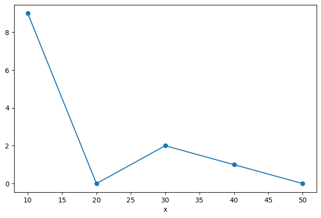
But things get most interesting when we add a coordinate:
da = xr.DataArray([9, 0, 2, 1, 0],
                  dims=['x'],
                  coords={'x': [10, 20, 30, 40, 50]})
da
<xarray.DataArray (x: 5)>
array([9, 0, 2, 1, 0])
Coordinates:
  * x        (x) int64 10 20 30 40 50
This coordinate has been used to create an index, which works very similar to a Pandas index. In fact, under the hood, Xarray just reuses Pandas indexes.
da.indexes
Indexes:
    x        Int64Index([10, 20, 30, 40, 50], dtype='int64', name='x')
Xarray has built-in plotting, like pandas.
da.plot(marker='o')
[<matplotlib.lines.Line2D at 0x7f9aae456f80>]
Multidimensional DataArray#
If we are just dealing with 1D data, Pandas and Xarray have very similar capabilities. Xarray’s real potential comes with multidimensional data.
Let’s go back to the multidimensional ARGO data we loaded in the numpy lesson.
import pooch
url = "https://www.ldeo.columbia.edu/~rpa/float_data_4901412.zip"
files = pooch.retrieve(url, processor=pooch.Unzip(), known_hash="2a703c720302c682f1662181d329c9f22f9f10e1539dc2d6082160a469165009")
files.sort()
files
['/home/jovyan/.cache/pooch/7e6685dbe2a3c0b0870f770f3ef413d9-float_data_4901412.zip.unzip/float_data/P.npy',
 '/home/jovyan/.cache/pooch/7e6685dbe2a3c0b0870f770f3ef413d9-float_data_4901412.zip.unzip/float_data/S.npy',
 '/home/jovyan/.cache/pooch/7e6685dbe2a3c0b0870f770f3ef413d9-float_data_4901412.zip.unzip/float_data/T.npy',
 '/home/jovyan/.cache/pooch/7e6685dbe2a3c0b0870f770f3ef413d9-float_data_4901412.zip.unzip/float_data/date.npy',
 '/home/jovyan/.cache/pooch/7e6685dbe2a3c0b0870f770f3ef413d9-float_data_4901412.zip.unzip/float_data/lat.npy',
 '/home/jovyan/.cache/pooch/7e6685dbe2a3c0b0870f770f3ef413d9-float_data_4901412.zip.unzip/float_data/levels.npy',
 '/home/jovyan/.cache/pooch/7e6685dbe2a3c0b0870f770f3ef413d9-float_data_4901412.zip.unzip/float_data/lon.npy']
We will manually load each of these variables into a numpy array. If this seems repetitive and inefficient, that’s the point! NumPy itself is not meant for managing groups of inter-related arrays. That’s what Xarray is for!
P = np.load(files[0])
S = np.load(files[1])
T = np.load(files[2])
date = np.load(files[3])
lat = np.load(files[4])
levels = np.load(files[5])
lon = np.load(files[6])
Let’s organize the data and coordinates of the salinity variable into a DataArray.
da_salinity = xr.DataArray(S, dims=['level', 'date'],
                           coords={'level': levels,
                                   'date': date},)
da_salinity
<xarray.DataArray (level: 78, date: 75)>
array([[35.6389389 , 35.51495743, 35.57297134, ..., 35.82093811,
35.77793884, 35.66891098],
[35.63393784, 35.5219574 , 35.57397079, ..., 35.81093216,
35.58389664, 35.66791153],
[35.6819458 , 35.52595901, 35.57297134, ..., 35.79592896,
35.66290665, 35.66591263],
...,
[34.91585922, 34.92390442, 34.92390442, ..., 34.93481064,
34.94081116, 34.94680786],
[34.91585922, 34.92390442, 34.92190552, ..., 34.93280792,
34.93680954, 34.94380951],
[34.91785812, 34.92390442, 34.92390442, ..., nan,
34.93680954, nan]])
Coordinates:
* level (level) int64 0 1 2 3 4 5 6 7 8 9 ... 68 69 70 71 72 73 74 75 76 77
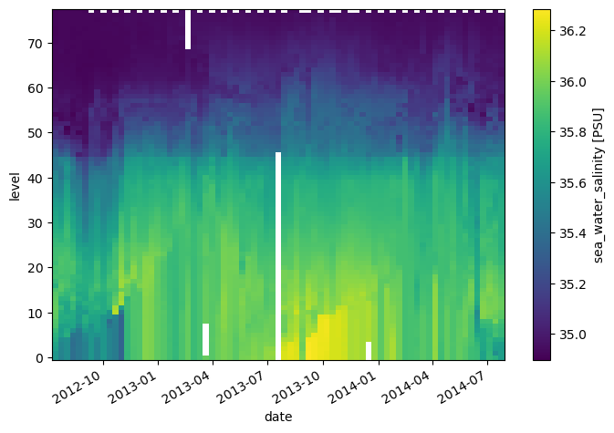
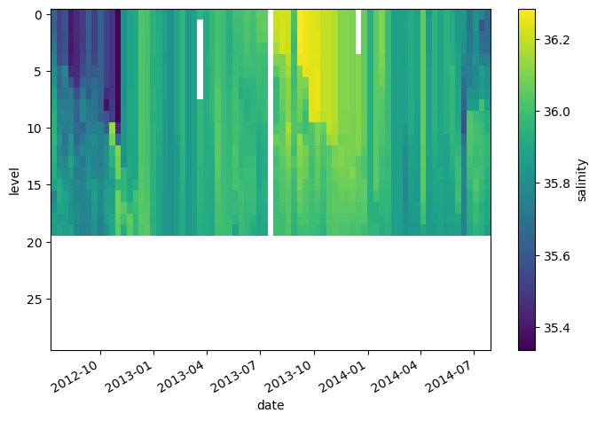
* date (date) datetime64[ns] 2012-07-13T22:33:06.019200 ... 2014-07-24T...da_salinity.plot(yincrease=False)
<matplotlib.collections.QuadMesh at 0x7f9a91aca530>
Attributes can be used to store metadata. What metadata should you store? The CF Conventions are a great resource for thinking about climate metadata. Below we define two of the required CF-conventions attributes.
da_salinity.attrs['units'] = 'PSU'
da_salinity.attrs['standard_name'] = 'sea_water_salinity'
da_salinity
<xarray.DataArray (level: 78, date: 75)>
array([[35.6389389 , 35.51495743, 35.57297134, ..., 35.82093811,
        35.77793884, 35.66891098],
       [35.63393784, 35.5219574 , 35.57397079, ..., 35.81093216,
        35.58389664, 35.66791153],
       [35.6819458 , 35.52595901, 35.57297134, ..., 35.79592896,
        35.66290665, 35.66591263],
       ...,
       [34.91585922, 34.92390442, 34.92390442, ..., 34.93481064,
        34.94081116, 34.94680786],
       [34.91585922, 34.92390442, 34.92190552, ..., 34.93280792,
        34.93680954, 34.94380951],
       [34.91785812, 34.92390442, 34.92390442, ...,         nan,
        34.93680954,         nan]])
Coordinates:
* level (level) int64 0 1 2 3 4 5 6 7 8 9 ... 68 69 70 71 72 73 74 75 76 77
* date (date) datetime64[ns] 2012-07-13T22:33:06.019200 ... 2014-07-24T...
Attributes:
units: PSU
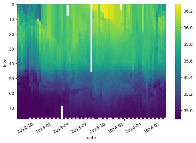
standard_name: sea_water_salinityNow if we plot the data again, the name and units are automatically attached to the figure.
da_salinity.plot()
<matplotlib.collections.QuadMesh at 0x7f9a91a14430>
Datasets#
A Dataset holds many DataArrays which potentially can share coordinates. In analogy to pandas:
pandas.Series : pandas.Dataframe :: xarray.DataArray : xarray.Dataset
Constructing Datasets manually is a bit more involved in terms of syntax. The Dataset constructor takes three arguments:
data_varsshould be a dictionary with each key as the name of the variable and each value as one of:A
DataArrayor VariableA tuple of the form
(dims, data[, attrs]), which is converted into arguments for VariableA pandas object, which is converted into a
DataArrayA 1D array or list, which is interpreted as values for a one dimensional coordinate variable along the same dimension as it’s name
coordsshould be a dictionary of the same form as data_vars.attrsshould be a dictionary.
Let’s put together a Dataset with temperature, salinity and pressure all together
argo = xr.Dataset(
    data_vars={
        'salinity':    (('level', 'date'), S),
        'temperature': (('level', 'date'), T),
        'pressure':    (('level', 'date'), P)
    },
    coords={
        'level': levels,
        'date': date
    }
)
argo
<xarray.Dataset>
Dimensions:      (level: 78, date: 75)
Coordinates:
  * level        (level) int64 0 1 2 3 4 5 6 7 8 ... 69 70 71 72 73 74 75 76 77
  * date         (date) datetime64[ns] 2012-07-13T22:33:06.019200 ... 2014-07...
Data variables:
    salinity     (level, date) float64 35.64 35.51 35.57 35.4 ... nan 34.94 nan
    temperature  (level, date) float64 18.97 18.44 19.1 19.79 ... nan 3.714 nan
pressure (level, date) float64 6.8 6.1 6.5 5.0 ... 2e+03 nan 2e+03 nanWhat about lon and lat? We forgot them in the creation process, but we can add them after the fact.
argo.coords['lon'] = lon
argo
<xarray.Dataset>
Dimensions:      (level: 78, date: 75, lon: 75)
Coordinates:
  * level        (level) int64 0 1 2 3 4 5 6 7 8 ... 69 70 71 72 73 74 75 76 77
  * date         (date) datetime64[ns] 2012-07-13T22:33:06.019200 ... 2014-07...
  * lon          (lon) float64 -39.13 -37.28 -36.9 ... -33.83 -34.11 -34.38
Data variables:
    salinity     (level, date) float64 35.64 35.51 35.57 35.4 ... nan 34.94 nan
    temperature  (level, date) float64 18.97 18.44 19.1 19.79 ... nan 3.714 nan
pressure (level, date) float64 6.8 6.1 6.5 5.0 ... 2e+03 nan 2e+03 nanThat was not quite right…we want lon to have dimension date:
del argo['lon']
argo.coords['lon'] = ('date', lon)
argo.coords['lat'] = ('date', lat)
argo
<xarray.Dataset>
Dimensions:      (level: 78, date: 75)
Coordinates:
  * level        (level) int64 0 1 2 3 4 5 6 7 8 ... 69 70 71 72 73 74 75 76 77
  * date         (date) datetime64[ns] 2012-07-13T22:33:06.019200 ... 2014-07...
    lon          (date) float64 -39.13 -37.28 -36.9 ... -33.83 -34.11 -34.38
    lat          (date) float64 47.19 46.72 46.45 46.23 ... 42.6 42.46 42.38
Data variables:
    salinity     (level, date) float64 35.64 35.51 35.57 35.4 ... nan 34.94 nan
    temperature  (level, date) float64 18.97 18.44 19.1 19.79 ... nan 3.714 nan
pressure (level, date) float64 6.8 6.1 6.5 5.0 ... 2e+03 nan 2e+03 nanCoordinates vs. Data Variables#
Data variables can be modified through arithmentic operations or other functions. Coordinates are always keept the same.
argo * 10000
<xarray.Dataset>
Dimensions:      (level: 78, date: 75)
Coordinates:
  * level        (level) int64 0 1 2 3 4 5 6 7 8 ... 69 70 71 72 73 74 75 76 77
  * date         (date) datetime64[ns] 2012-07-13T22:33:06.019200 ... 2014-07...
    lon          (date) float64 -39.13 -37.28 -36.9 ... -33.83 -34.11 -34.38
    lat          (date) float64 47.19 46.72 46.45 46.23 ... 42.6 42.46 42.38
Data variables:
    salinity     (level, date) float64 3.564e+05 3.551e+05 ... 3.494e+05 nan
    temperature  (level, date) float64 1.897e+05 1.844e+05 ... 3.714e+04 nan
pressure (level, date) float64 6.8e+04 6.1e+04 6.5e+04 ... nan 2e+07 nanClearly lon and lat are coordinates rather than data variables. We can change their status as follows:
argo = argo.set_coords(['lon', 'lat'])
argo
<xarray.Dataset>
Dimensions:      (level: 78, date: 75)
Coordinates:
  * level        (level) int64 0 1 2 3 4 5 6 7 8 ... 69 70 71 72 73 74 75 76 77
  * date         (date) datetime64[ns] 2012-07-13T22:33:06.019200 ... 2014-07...
    lon          (date) float64 -39.13 -37.28 -36.9 ... -33.83 -34.11 -34.38
    lat          (date) float64 47.19 46.72 46.45 46.23 ... 42.6 42.46 42.38
Data variables:
    salinity     (level, date) float64 35.64 35.51 35.57 35.4 ... nan 34.94 nan
    temperature  (level, date) float64 18.97 18.44 19.1 19.79 ... nan 3.714 nan
pressure (level, date) float64 6.8 6.1 6.5 5.0 ... 2e+03 nan 2e+03 nanThe * symbol in the representation above indicates that level and date are “dimension coordinates” (they describe the coordinates associated with data variable axes) while lon and lat are “non-dimension coordinates”. We can make any variable a non-dimension coordiante.
Alternatively, we could have assigned directly to coords as follows:
argo.coords['lon'] = ('date', lon)
argo.coords['lat'] = ('date', lat)
Selecting Data (Indexing)#
We can always use regular numpy indexing and slicing on DataArrays
argo.salinity[2]
<xarray.DataArray 'salinity' (date: 75)>
array([35.6819458 , 35.52595901, 35.57297134, 35.40494537, 35.45091629,
       35.50192261, 35.62397766, 35.51696014, 35.62797546, 35.52292252,
       35.47383118, 35.33785629, 35.81896591, 35.88694   , 35.90187836,
       36.02391815, 36.00475693, 35.94187927, 35.91583252, 35.86392212,
       35.81995392, 35.88601303, 35.95079422, 35.84091568, 35.87992477,
               nan, 35.92179108, 35.96979141, 36.0008316 , 35.98083115,
       35.92887878, 35.98091888, 35.9838829 , 36.01884842, 35.99092484,
       36.04689026, 36.04185867,         nan, 36.19193268, 36.22789764,
       36.20986557, 35.97589874, 36.2779007 , 36.25889969, 36.2418251 ,
       36.23685837, 36.19781876, 36.19785309, 36.17692184, 36.1048851 ,
       36.11392212, 36.09080505,         nan, 36.05675888, 35.93374634,
       36.04291534, 36.10183716, 35.97779083, 35.86592102, 35.87791824,
       35.88392258, 35.92078781, 35.88601303, 36.05178833, 35.85883713,
       35.94878769, 35.8938446 , 35.94379425, 35.90884018, 35.84893036,
       35.83496857, 35.71691132, 35.79592896, 35.66290665, 35.66591263])
Coordinates:
    level    int64 2
  * date     (date) datetime64[ns] 2012-07-13T22:33:06.019200 ... 2014-07-24T...
    lon      (date) float64 -39.13 -37.28 -36.9 -36.89 ... -33.83 -34.11 -34.38
lat (date) float64 47.19 46.72 46.45 46.23 ... 42.72 42.6 42.46 42.38argo.salinity[2].plot()
[<matplotlib.lines.Line2D at 0x7f9a91929960>]
argo.salinity[:, 10]
<xarray.DataArray 'salinity' (level: 78)>
array([35.47483063, 35.47483063, 35.47383118, 35.47383118, 35.47383118,
35.47483063, 35.48183441, 35.47983551, 35.4948349 , 35.51083755,
36.13380051, 36.09579849, 35.95479965, 35.93979645, 35.8958931 ,
35.86388397, 35.87788773, 35.88188934, 35.90379333, 35.9067955 ,
35.86588669, 35.8588829 , 35.86088181, 35.85188293, 35.85788345,
35.82787323, 35.78786469, 35.73185349, 35.69784927, 35.67684174,
35.677845 , 35.65784073, 35.64083481, 35.6238327 , 35.59682846,
35.57782364, 35.56182098, 35.55781937, 35.52181625, 35.49881363,
35.51381302, 35.49981308, 35.47280884, 35.47880936, 35.44780731,
35.39379501, 35.35879135, 35.28778076, 35.21878052, 35.20677567,
35.17777252, 35.15076828, 35.07276535, 35.01475525, 34.9797554 ,
35.0117569 , 35.03975677, 35.05575562, 35.00975037, 34.96175385,
34.96775055, 34.95075226, 34.93775177, 34.93375015, 34.93775558,
34.9247551 , 34.92175674, 34.91975403, 34.91975403, 34.91975403,
34.92176056, 34.92375946, 34.92575836, 34.92575836, 34.92475891,
34.93076324, 34.92176437, nan])
Coordinates:
* level (level) int64 0 1 2 3 4 5 6 7 8 9 ... 68 69 70 71 72 73 74 75 76 77
date datetime64[ns] 2012-10-22T02:50:32.006400
lon float64 -32.97
lat float64 44.13argo.salinity[:, 10].plot()
[<matplotlib.lines.Line2D at 0x7f9a917b30a0>]
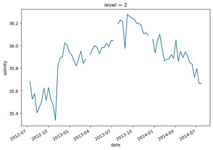
However, it is often much more powerful to use xarray’s .sel() method to use label-based indexing.
argo.salinity.sel(level=2)
<xarray.DataArray 'salinity' (date: 75)>
array([35.6819458 , 35.52595901, 35.57297134, 35.40494537, 35.45091629,
       35.50192261, 35.62397766, 35.51696014, 35.62797546, 35.52292252,
       35.47383118, 35.33785629, 35.81896591, 35.88694   , 35.90187836,
       36.02391815, 36.00475693, 35.94187927, 35.91583252, 35.86392212,
       35.81995392, 35.88601303, 35.95079422, 35.84091568, 35.87992477,
               nan, 35.92179108, 35.96979141, 36.0008316 , 35.98083115,
       35.92887878, 35.98091888, 35.9838829 , 36.01884842, 35.99092484,
       36.04689026, 36.04185867,         nan, 36.19193268, 36.22789764,
       36.20986557, 35.97589874, 36.2779007 , 36.25889969, 36.2418251 ,
       36.23685837, 36.19781876, 36.19785309, 36.17692184, 36.1048851 ,
       36.11392212, 36.09080505,         nan, 36.05675888, 35.93374634,
       36.04291534, 36.10183716, 35.97779083, 35.86592102, 35.87791824,
       35.88392258, 35.92078781, 35.88601303, 36.05178833, 35.85883713,
       35.94878769, 35.8938446 , 35.94379425, 35.90884018, 35.84893036,
       35.83496857, 35.71691132, 35.79592896, 35.66290665, 35.66591263])
Coordinates:
level int64 2
* date (date) datetime64[ns] 2012-07-13T22:33:06.019200 ... 2014-07-24T...
lon (date) float64 -39.13 -37.28 -36.9 -36.89 ... -33.83 -34.11 -34.38
lat (date) float64 47.19 46.72 46.45 46.23 ... 42.72 42.6 42.46 42.38argo.salinity.sel(level=2).plot()
[<matplotlib.lines.Line2D at 0x7f9a918404f0>]

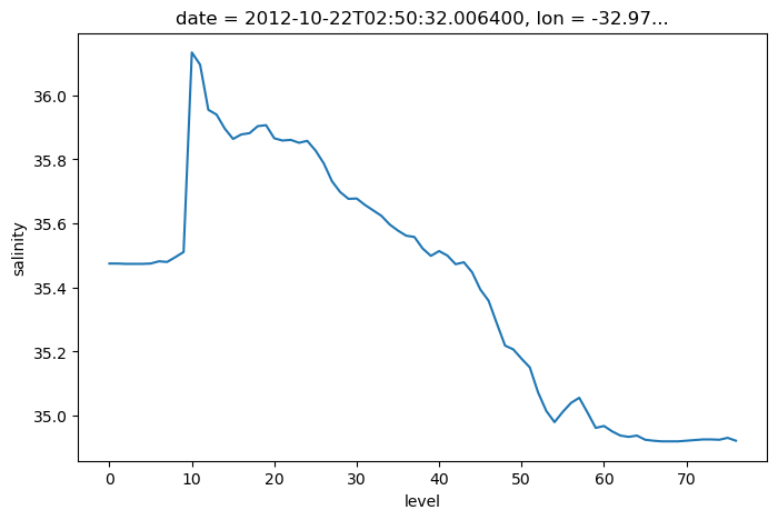
argo.salinity.sel(date='2012-10-22')
<xarray.DataArray 'salinity' (level: 78, date: 1)>
array([[35.47483063],
       [35.47483063],
       [35.47383118],
       [35.47383118],
       [35.47383118],
       [35.47483063],
       [35.48183441],
       [35.47983551],
       [35.4948349 ],
       [35.51083755],
       [36.13380051],
       [36.09579849],
       [35.95479965],
       [35.93979645],
       [35.8958931 ],
       [35.86388397],
       [35.87788773],
       [35.88188934],
       [35.90379333],
       [35.9067955 ],
...
       [35.00975037],
       [34.96175385],
       [34.96775055],
       [34.95075226],
       [34.93775177],
       [34.93375015],
       [34.93775558],
       [34.9247551 ],
       [34.92175674],
       [34.91975403],
       [34.91975403],
       [34.91975403],
       [34.92176056],
       [34.92375946],
       [34.92575836],
       [34.92575836],
       [34.92475891],
       [34.93076324],
       [34.92176437],
       [        nan]])
Coordinates:
  * level    (level) int64 0 1 2 3 4 5 6 7 8 9 ... 68 69 70 71 72 73 74 75 76 77
  * date     (date) datetime64[ns] 2012-10-22T02:50:32.006400
    lon      (date) float64 -32.97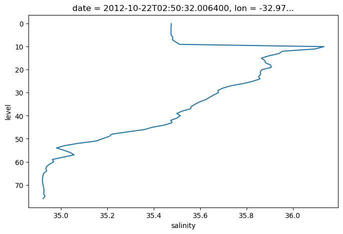
lat (date) float64 44.13argo.salinity.sel(date='2012-10-22').plot(y='level', yincrease=False)
[<matplotlib.lines.Line2D at 0x7f9a916d24a0>]
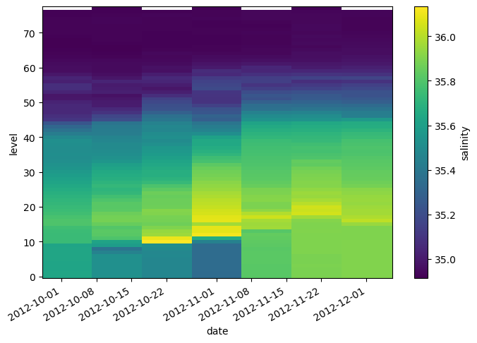
.sel() also supports slicing. Unfortunately we have to use a somewhat awkward syntax, but it still works.
argo.salinity.sel(date=slice('2012-10-01', '2012-12-01'))
<xarray.DataArray 'salinity' (level: 78, date: 7)>
array([[35.63097763, 35.52592468, 35.47483063, 35.33785629, 35.81896591,
        35.8889389 , 35.90187836],
       [35.63097763, 35.52292252, 35.47483063, 35.33685684, 35.81796646,
        35.88793945, 35.90187836],
       [35.62797546, 35.52292252, 35.47383118, 35.33785629, 35.81896591,
        35.88694   , 35.90187836],
       [35.62697601, 35.52192307, 35.47383118, 35.33785629, 35.81896591,
        35.89193726, 35.90187836],
       [35.62797546, 35.52192307, 35.47383118, 35.33785629, 35.81996536,
        35.88993835, 35.90187836],
       [35.62897873, 35.52292252, 35.47483063, 35.33785629, 35.81996536,
        35.88993835, 35.90187836],
       [35.62997818, 35.51892471, 35.48183441, 35.33785629, 35.81996536,
        35.88993835, 35.90187836],
       [35.63197708, 35.44991302, 35.47983551, 35.33785629, 35.81996536,
        35.89683914, 35.90187836],
       [35.63097763, 35.38090134, 35.4948349 , 35.33785629, 35.81896591,
        35.89583969, 35.90187836],
       [35.62697601, 35.58792114, 35.51083755, 35.33985519, 35.82497025,
        35.89683914, 35.90187836],
...
       [34.91690445, 34.92385483, 34.91975403, 34.91980362, 34.92385483,
        34.93680573, 34.93885422],
       [34.92190552, 34.92485428, 34.91975403, 34.92080688, 34.92485428,
        34.94480515, 34.9328537 ],
       [34.92390442, 34.92285538, 34.92176056, 34.92280579, 34.92985535,
        34.93280411, 34.92785645],
       [34.92390442, 34.92385483, 34.92375946, 34.92480469, 34.92685318,
        34.93780899, 34.92485428],
       [34.92390442, 34.92285538, 34.92575836, 34.92181015, 34.92085648,
        34.93680954, 34.92385483],
       [34.92590332, 34.9288559 , 34.92575836, 34.92181015, 34.92685318,
        34.93481064, 34.92585373],
       [34.92490387, 34.92785645, 34.92475891, 34.92781067, 34.93385696,
        34.93380737, 34.92385864],
       [34.92190552, 34.92385864, 34.93076324, 34.9268074 , 34.93585968,
        34.93481064, 34.92985916],
       [34.92090607, 34.92185974, 34.92176437, 34.9228096 , 34.93285751,
        34.93180847, 34.92786026],
       [        nan, 34.91985703,         nan, 34.92181015,         nan,
        34.92181015,         nan]])
Coordinates:
  * level    (level) int64 0 1 2 3 4 5 6 7 8 9 ... 68 69 70 71 72 73 74 75 76 77
  * date     (date) datetime64[ns] 2012-10-02T03:00:17.971200 ... 2012-12-01T...
    lon      (date) float64 -34.46 -33.78 -32.97 -32.55 -32.43 -32.29 -32.17
lat (date) float64 44.96 44.68 44.13 43.64 43.07 42.66 42.51argo.salinity.sel(date=slice('2012-10-01', '2012-12-01')).plot()
<matplotlib.collections.QuadMesh at 0x7f9a9172aad0>
.sel() also works on the whole Dataset
argo.sel(date='2012-10-22')
<xarray.Dataset>
Dimensions:      (level: 78, date: 1)
Coordinates:
  * level        (level) int64 0 1 2 3 4 5 6 7 8 ... 69 70 71 72 73 74 75 76 77
  * date         (date) datetime64[ns] 2012-10-22T02:50:32.006400
    lon          (date) float64 -32.97
    lat          (date) float64 44.13
Data variables:
    salinity     (level, date) float64 35.47 35.47 35.47 ... 34.93 34.92 nan
    temperature  (level, date) float64 17.13 17.13 17.13 ... 3.736 3.639 nan
pressure (level, date) float64 6.4 10.3 15.4 ... 1.9e+03 1.951e+03 nanComputation#
Xarray dataarrays and datasets work seamlessly with arithmetic operators and numpy array functions.
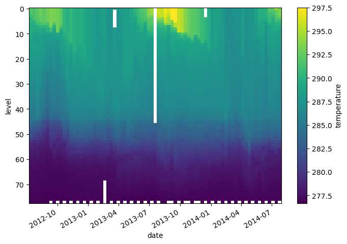
temp_kelvin = argo.temperature + 273.15
temp_kelvin.plot(yincrease=False)
<matplotlib.collections.QuadMesh at 0x7f9a9160b400>
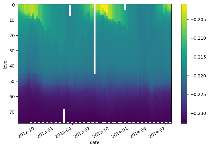
We can also combine multiple xarray datasets in arithemtic operations
g = 9.8
buoyancy = g * (2e-4 * argo.temperature - 7e-4 * argo.salinity)
buoyancy.plot(yincrease=False)
<matplotlib.collections.QuadMesh at 0x7f9a9150d4b0>
Broadcasting, Aligment, and Combining Data#
Broadcasting#
Broadcasting arrays in numpy is a nightmare. It is much easier when the data axes are labeled!
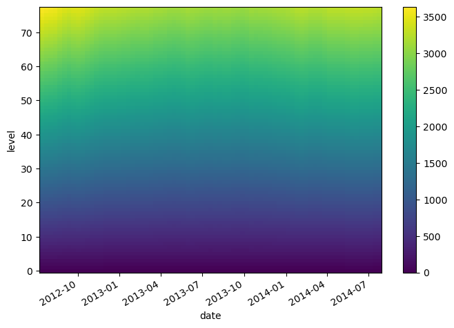
This is a useless calculation, but it illustrates how perfoming an operation on arrays with differenty coordinates will result in automatic broadcasting
level_times_lat = argo.level * argo.lat
level_times_lat
<xarray.DataArray (level: 78, date: 75)>
array([[   0.   ,    0.   ,    0.   , ...,    0.   ,    0.   ,    0.   ],
       [  47.187,   46.716,   46.45 , ...,   42.601,   42.457,   42.379],
       [  94.374,   93.432,   92.9  , ...,   85.202,   84.914,   84.758],
       ...,
       [3539.025, 3503.7  , 3483.75 , ..., 3195.075, 3184.275, 3178.425],
       [3586.212, 3550.416, 3530.2  , ..., 3237.676, 3226.732, 3220.804],
       [3633.399, 3597.132, 3576.65 , ..., 3280.277, 3269.189, 3263.183]])
Coordinates:
  * level    (level) int64 0 1 2 3 4 5 6 7 8 9 ... 68 69 70 71 72 73 74 75 76 77
  * date     (date) datetime64[ns] 2012-07-13T22:33:06.019200 ... 2014-07-24T...
    lon      (date) float64 -39.13 -37.28 -36.9 -36.89 ... -33.83 -34.11 -34.38
lat (date) float64 47.19 46.72 46.45 46.23 ... 42.72 42.6 42.46 42.38level_times_lat.plot()
<matplotlib.collections.QuadMesh at 0x7f9a913e9cc0>
Alignment#
If you try to perform operations on DataArrays that share a dimension name, Xarray will try to align them first. This works nearly identically to Pandas, except that there can be multiple dimensions to align over.
To see how alignment works, we will create some subsets of our original data.
sa_surf = argo.salinity.isel(level=slice(0, 20))
sa_mid = argo.salinity.isel(level=slice(10, 30))
By default, when we combine multiple arrays in mathematical operations, Xarray performs an “inner join”.
(sa_surf * sa_mid).level
<xarray.DataArray 'level' (level: 10)>
array([10, 11, 12, 13, 14, 15, 16, 17, 18, 19])
Coordinates:
  * level    (level) int64 10 11 12 13 14 15 16 17 18 19
We can override this behavior by manually aligning the data
sa_surf_outer, sa_mid_outer = xr.align(sa_surf, sa_mid, join='outer')
sa_surf_outer.level
<xarray.DataArray 'level' (level: 30)>
array([ 0,  1,  2,  3,  4,  5,  6,  7,  8,  9, 10, 11, 12, 13, 14, 15, 16, 17,
       18, 19, 20, 21, 22, 23, 24, 25, 26, 27, 28, 29])
Coordinates:
* level (level) int64 0 1 2 3 4 5 6 7 8 9 ... 20 21 22 23 24 25 26 27 28 29As we can see, missing data (NaNs) have been filled in where the array was extended.
sa_surf_outer.plot(yincrease=False)
<matplotlib.collections.QuadMesh at 0x7f9a912bf6d0>
We can also use join='right' and join='left'.
Combing Data: Concat and Merge#
The ability to combine many smaller arrays into a single big Dataset is one of the main advantages of Xarray. To take advantage of this, we need to learn two operations that help us combine data:
xr.contact: to concatenate multiple arrays into one bigger array along their dimensionsxr.merge: to combine multiple different arrays into a dataset
First let’s look at concat. Let’s re-combine the subsetted data from the previous step.
sa_surf_mid = xr.concat([sa_surf, sa_mid], dim='level')
sa_surf_mid
<xarray.DataArray 'salinity' (level: 40, date: 75)>
array([[35.6389389 , 35.51495743, 35.57297134, ..., 35.82093811,
        35.77793884, 35.66891098],
       [35.63393784, 35.5219574 , 35.57397079, ..., 35.81093216,
        35.58389664, 35.66791153],
       [35.6819458 , 35.52595901, 35.57297134, ..., 35.79592896,
        35.66290665, 35.66591263],
       ...,
       [35.78895187, 35.7829895 , 35.85100555, ..., 35.84291458,
        35.81891251, 35.7779007 ],
       [35.76794815, 35.75598526, 35.84500504, ..., 35.84891891,
        35.83391571, 35.76390076],
       [35.75194168, 35.71097565, 35.83100128, ..., 35.80690765,
        35.85292053, 35.75489807]])
Coordinates:
  * level    (level) int64 0 1 2 3 4 5 6 7 8 9 ... 20 21 22 23 24 25 26 27 28 29
  * date     (date) datetime64[ns] 2012-07-13T22:33:06.019200 ... 2014-07-24T...
    lon      (date) float64 -39.13 -37.28 -36.9 -36.89 ... -33.83 -34.11 -34.38
lat (date) float64 47.19 46.72 46.45 46.23 ... 42.72 42.6 42.46 42.38Warning
Xarray won’t check the values of the coordinates before concat. It will just stick everything together into a new array.
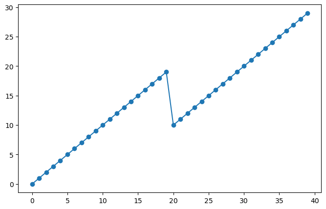
In this case, we had overlapping data. We can see this by looking at the level coordinate.
sa_surf_mid.level
<xarray.DataArray 'level' (level: 40)>
array([ 0,  1,  2,  3,  4,  5,  6,  7,  8,  9, 10, 11, 12, 13, 14, 15, 16, 17,
       18, 19, 10, 11, 12, 13, 14, 15, 16, 17, 18, 19, 20, 21, 22, 23, 24, 25,
       26, 27, 28, 29])
Coordinates:
* level (level) int64 0 1 2 3 4 5 6 7 8 9 ... 20 21 22 23 24 25 26 27 28 29plt.plot(sa_surf_mid.level.values, marker='o')
[<matplotlib.lines.Line2D at 0x7f9a91a9fc70>]
We can also concat data along a new dimension, e.g.
sa_concat_new = xr.concat([sa_surf, sa_mid], dim='newdim')
sa_concat_new
<xarray.DataArray 'salinity' (newdim: 2, level: 30, date: 75)>
array([[[35.6389389 , 35.51495743, 35.57297134, ..., 35.82093811,
         35.77793884, 35.66891098],
        [35.63393784, 35.5219574 , 35.57397079, ..., 35.81093216,
         35.58389664, 35.66791153],
        [35.6819458 , 35.52595901, 35.57297134, ..., 35.79592896,
         35.66290665, 35.66591263],
        ...,
        [        nan,         nan,         nan, ...,         nan,
                 nan,         nan],
        [        nan,         nan,         nan, ...,         nan,
                 nan,         nan],
        [        nan,         nan,         nan, ...,         nan,
                 nan,         nan]],

       [[        nan,         nan,         nan, ...,         nan,
                 nan,         nan],
        [        nan,         nan,         nan, ...,         nan,
                 nan,         nan],
        [        nan,         nan,         nan, ...,         nan,
                 nan,         nan],
        ...,
        [35.78895187, 35.7829895 , 35.85100555, ..., 35.84291458,
         35.81891251, 35.7779007 ],
        [35.76794815, 35.75598526, 35.84500504, ..., 35.84891891,
         35.83391571, 35.76390076],
        [35.75194168, 35.71097565, 35.83100128, ..., 35.80690765,
         35.85292053, 35.75489807]]])
Coordinates:
  * level    (level) int64 0 1 2 3 4 5 6 7 8 9 ... 20 21 22 23 24 25 26 27 28 29
  * date     (date) datetime64[ns] 2012-07-13T22:33:06.019200 ... 2014-07-24T...
    lon      (date) float64 -39.13 -37.28 -36.9 -36.89 ... -33.83 -34.11 -34.38
    lat      (date) float64 47.19 46.72 46.45 46.23 ... 42.72 42.6 42.46 42.38
Dimensions without coordinates: newdimNote that the data were aligned using an outer join along the non-concat dimensions.
Instead of specifying a new dimension name, we can pass a new Pandas index object explicitly to concat.
This will create a new dimension coordinate and corresponding index.
We can merge both DataArrays and Datasets.
xr.merge([argo.salinity, argo.temperature])
<xarray.Dataset>
Dimensions:      (level: 78, date: 75)
Coordinates:
  * level        (level) int64 0 1 2 3 4 5 6 7 8 ... 69 70 71 72 73 74 75 76 77
  * date         (date) datetime64[ns] 2012-07-13T22:33:06.019200 ... 2014-07...
    lon          (date) float64 -39.13 -37.28 -36.9 ... -33.83 -34.11 -34.38
    lat          (date) float64 47.19 46.72 46.45 46.23 ... 42.6 42.46 42.38
Data variables:
    salinity     (level, date) float64 35.64 35.51 35.57 35.4 ... nan 34.94 nan
temperature (level, date) float64 18.97 18.44 19.1 19.79 ... nan 3.714 nanIf the data are not aligned, they will be aligned before merge.
We can specify the join options in merge.
xr.merge([
    argo.salinity.sel(level=slice(0, 30)),
    argo.temperature.sel(level=slice(30, None))
])
<xarray.Dataset>
Dimensions:      (level: 78, date: 75)
Coordinates:
  * level        (level) int64 0 1 2 3 4 5 6 7 8 ... 69 70 71 72 73 74 75 76 77
  * date         (date) datetime64[ns] 2012-07-13T22:33:06.019200 ... 2014-07...
    lon          (date) float64 -39.13 -37.28 -36.9 ... -33.83 -34.11 -34.38
    lat          (date) float64 47.19 46.72 46.45 46.23 ... 42.6 42.46 42.38
Data variables:
    salinity     (level, date) float64 35.64 35.51 35.57 35.4 ... nan nan nan
temperature (level, date) float64 nan nan nan nan ... 3.728 nan 3.714 nanxr.merge([
argo.salinity.sel(level=slice(0, 30)),
argo.temperature.sel(level=slice(30, None))
], join='left')
<xarray.Dataset>
Dimensions:      (level: 31, date: 75)
Coordinates:
  * level        (level) int64 0 1 2 3 4 5 6 7 8 ... 22 23 24 25 26 27 28 29 30
  * date         (date) datetime64[ns] 2012-07-13T22:33:06.019200 ... 2014-07...
    lon          (date) float64 -39.13 -37.28 -36.9 ... -33.83 -34.11 -34.38
    lat          (date) float64 47.19 46.72 46.45 46.23 ... 42.6 42.46 42.38
Data variables:
    salinity     (level, date) float64 35.64 35.51 35.57 ... 35.78 35.83 35.76
temperature (level, date) float64 nan nan nan nan ... 13.59 13.74 13.31Reductions#
Just like in numpy, we can reduce xarray DataArrays along any number of axes:
argo.temperature.mean(axis=0)
<xarray.DataArray 'temperature' (date: 75)>
array([10.88915385, 10.7282564 , 10.9336282 , 10.75679484, 10.38166666,
       10.08619236, 10.58194804, 10.50066671, 10.56841555, 10.53705122,
       10.81131168, 11.01932052, 11.39205196, 11.40823073, 11.3642208 ,
       11.35821797, 11.39444157, 11.10514098, 11.02870125, 10.80894868,
       10.93076625, 11.01069231, 11.88195654, 10.57373078, 10.66359736,
       10.56573237, 11.08854546, 10.87921792, 11.21384416, 11.24991028,
       11.29168825, 11.06203848, 11.32829864, 11.20401279, 11.25300001,
       11.32106403, 11.40112986,  6.07053117, 11.7748052 , 11.7466795 ,
       12.03732056, 11.92653251, 12.08844156, 12.20543591, 12.23402598,
       12.03365387, 11.9919221 , 11.92087012, 11.84273071, 11.79711684,
       11.7895325 , 11.55385894, 11.19083561, 11.266282  , 11.0611948 ,
       11.0307179 , 11.06566232, 10.79799995, 10.787     , 10.41173077,
       10.44170127, 10.32649998, 10.38242857, 10.88080769, 10.86177921,
       10.98787178, 10.93602596, 10.73039743, 11.09251948, 10.93983334,
       10.65942862, 11.01814097, 11.21918184, 11.19080765, 11.13364934])
Coordinates:
  * date     (date) datetime64[ns] 2012-07-13T22:33:06.019200 ... 2014-07-24T...
    lon      (date) float64 -39.13 -37.28 -36.9 -36.89 ... -33.83 -34.11 -34.38
lat (date) float64 47.19 46.72 46.45 46.23 ... 42.72 42.6 42.46 42.38argo.temperature.mean(axis=1)
<xarray.DataArray 'temperature' (level: 78)>
array([17.60172602, 17.57223609, 17.5145833 , 17.42326395, 17.24943838,
       17.03730134, 16.76787661, 16.44609588, 16.17439195, 16.04501356,
       15.65827023, 15.4607296 , 15.26114862, 15.12489191, 14.99133783,
       14.90160808, 14.81990544, 14.74535139, 14.66822971, 14.585027  ,
       14.49732434, 14.41904053, 14.35412163, 14.27102702, 14.19081082,
       14.11487838, 14.04347293, 13.98067566, 13.90994595, 13.83274319,
       13.76139196, 13.69836479, 13.62335132, 13.54185131, 13.46647295,
       13.39395946, 13.32541891, 13.25205403, 13.18131082, 13.10233782,
       12.89268916, 12.67795943, 12.4649189 , 12.2178513 , 11.98270268,
       11.1281081 , 10.80430666, 10.49702667, 10.1749066 ,  9.83453334,
        9.48625332,  9.19793334,  8.66010666,  8.12324001,  7.60221333,
        7.15289333,  6.74250667,  6.39543999,  6.04598667,  5.74538665,
        5.48913333,  5.26604001,  5.08768   ,  4.93479998,  4.77769334,
        4.65368   ,  4.54237334,  4.44274664,  4.35933333,  4.2653784 ,
        4.17290539,  4.08902703,  3.99864865,  3.92163514,  3.85617567,
        3.78916217,  3.72950001,  3.66207691])
Coordinates:
* level (level) int64 0 1 2 3 4 5 6 7 8 9 ... 68 69 70 71 72 73 74 75 76 77However, rather than performing reductions on axes (as in numpy), we can perform them on dimensions. This turns out to be a huge convenience
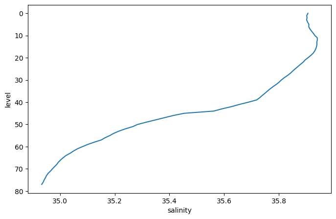
argo_mean = argo.mean(dim='date')
argo_mean
<xarray.Dataset>
Dimensions:      (level: 78)
Coordinates:
  * level        (level) int64 0 1 2 3 4 5 6 7 8 ... 69 70 71 72 73 74 75 76 77
Data variables:
    salinity     (level) float64 35.91 35.9 35.9 35.9 ... 34.94 34.94 34.93
    temperature  (level) float64 17.6 17.57 17.51 17.42 ... 3.789 3.73 3.662
pressure (level) float64 6.435 10.57 15.54 ... 1.95e+03 1.999e+03argo_mean.salinity.plot(y='level', yincrease=False)
[<matplotlib.lines.Line2D at 0x7f9a91266560>]
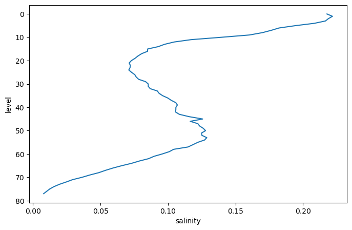
argo_std = argo.std(dim='date')
argo_std.salinity.plot(y='level', yincrease=False)
[<matplotlib.lines.Line2D at 0x7f9a910f5030>]
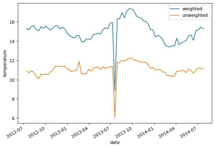
Weighted Reductions#
Sometimes we want to perform a reduction (e.g. a mean) where we assign different weight factors to each point in the array. Xarray supports this via weighted array reductions.
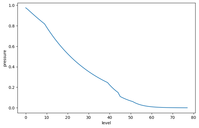
As a toy example, imagine we want to weight values in the upper ocean more than the lower ocean. We could imagine creating a weight array exponentially proportional to pressure as follows:
mean_pressure = argo.pressure.mean(dim='date')
p0 = 250  # dbat
weights = np.exp(-mean_pressure / p0)
weights.plot()
[<matplotlib.lines.Line2D at 0x7f9a91153910>]
The weighted mean over the level dimensions is calculated as follows:
temp_weighted_mean = argo.temperature.weighted(weights).mean('level')
Comparing to the unweighted mean, we see the difference:
temp_weighted_mean.plot(label='weighted')
argo.temperature.mean(dim='level').plot(label='unweighted')
plt.legend()
<matplotlib.legend.Legend at 0x7f9a90fc6770>
Loading Data from netCDF Files#
NetCDF (Network Common Data Format) is the most widely used format for distributing geoscience data. NetCDF is maintained by the Unidata organization.
Below we quote from the NetCDF website:
NetCDF (network Common Data Form) is a set of interfaces for array-oriented data access and a freely distributed collection of data access libraries for C, Fortran, C++, Java, and other languages. The netCDF libraries support a machine-independent format for representing scientific data. Together, the interfaces, libraries, and format support the creation, access, and sharing of scientific data.
NetCDF data is:
Self-Describing. A netCDF file includes information about the data it contains.
Portable. A netCDF file can be accessed by computers with different ways of storing integers, characters, and floating-point numbers.
Scalable. A small subset of a large dataset may be accessed efficiently.
Appendable. Data may be appended to a properly structured netCDF file without copying the dataset or redefining its structure.
Sharable. One writer and multiple readers may simultaneously access the same netCDF file.
Archivable. Access to all earlier forms of netCDF data will be supported by current and future versions of the software.
Xarray was designed to make reading netCDF files in python as easy, powerful, and flexible as possible. (See xarray netCDF docs for more details.)
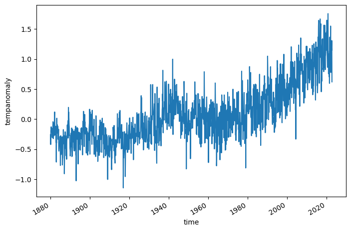
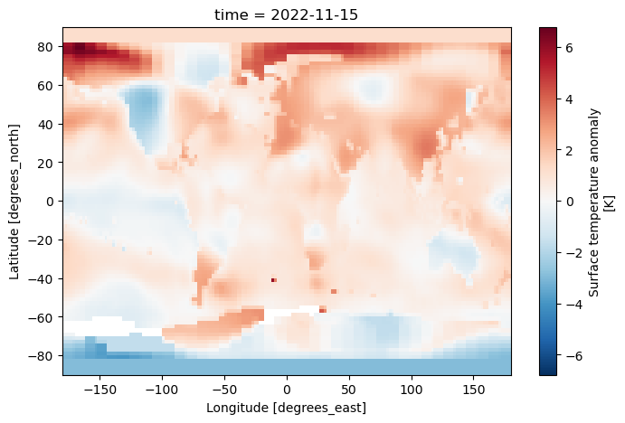
Below we download and load some the NASA GISSTemp global temperature anomaly dataset.
gistemp_file = pooch.retrieve(
    'https://data.giss.nasa.gov/pub/gistemp/gistemp1200_GHCNv4_ERSSTv5.nc.gz',
    known_hash='52e5c2d0b601ccb5188301ca5247b0563c0000dc6086dffa8489e555a109f3d0',
    processor=pooch.Decompress(),
)
ds = xr.open_dataset(gistemp_file)
ds
<xarray.Dataset>
Dimensions: (lat: 90, lon: 180, time: 1715, nv: 2)
Coordinates:
* lat (lat) float32 -89.0 -87.0 -85.0 -83.0 ... 83.0 85.0 87.0 89.0
* lon (lon) float32 -179.0 -177.0 -175.0 -173.0 ... 175.0 177.0 179.0
* time (time) datetime64[ns] 1880-01-15 1880-02-15 ... 2022-11-15
Dimensions without coordinates: nv
Data variables:
time_bnds (time, nv) datetime64[ns] ...
tempanomaly (time, lat, lon) float32 ...
Attributes:
title: GISTEMP Surface Temperature Analysis
institution: NASA Goddard Institute for Space Studies
source: http://data.giss.nasa.gov/gistemp/
Conventions: CF-1.6
history: Created 2022-12-12 11:35:15 by SBBX_to_nc 2.0 - ILAND=1200,...ds.tempanomaly.isel(time=-1).plot()
<matplotlib.collections.QuadMesh at 0x7f9a875fd810>
ds.tempanomaly.mean(dim=('lon', 'lat')).plot()
[<matplotlib.lines.Line2D at 0x7f9a8722bbe0>]