Maps in Scientific Python
Contents
Maps in Scientific Python#
Making maps is a fundamental part of geoscience research. Maps differ from regular figures in the following principle ways:
Maps require a projection of geographic coordinates on the 3D Earth to the 2D space of your figure.
Maps often include extra decorations besides just our data (e.g. continents, country borders, etc.)
Mapping is a notoriously hard and complicated problem, mostly due to the complexities of projection.
In this lecture, we will learn about Cartopy, one of the most common packages for making maps within python. Another popular and powerful library is Basemap; however, Basemap is going away and being replaced with Cartopy in the near future. For this reason, new python learners are recommended to learn Cartopy.
Credit: Phil Elson#
Lots of the material in this lesson was adopted from Phil Elson’s excellent Cartopy Tutorial. Phil is the creator of Cartopy and published his tutorial under an open license, meaning that we can copy, adapt, and redistribute it as long as we give proper attribution. THANKS PHIL! 👏👏👏
Background: Projections#
Most of our media for visualization are flat#
Our two most common media are flat:
Paper
Screen

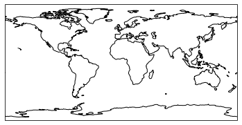
[Map] Projections: Taking us from spherical to flat#
A map projection (or more commonly refered to as just “projection”) is:
a systematic transformation of the latitudes and longitudes of locations from the surface of a sphere or an ellipsoid into locations on a plane. [Wikipedia: Map projection].
The major problem with map projections#
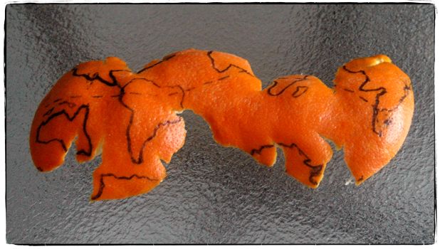
The surface of a sphere is topologically different to a 2D surface, therefore we have to cut the sphere somewhere
A sphere’s surface cannot be represented on a plane without distortion.
There are many different ways to make a projection, and we will not attempt to explain all of the choices and tradeoffs here. Instead, you can read Phil’s original tutorial for a great overview of this topic. Instead, we will dive into the more practical sides of Caropy usage.
Introducing Cartopy#
https://scitools.org.uk/cartopy/docs/latest/
Cartopy makes use of the powerful PROJ.4, numpy and shapely libraries and includes a programatic interface built on top of Matplotlib for the creation of publication quality maps.
Key features of cartopy are its object oriented projection definitions, and its ability to transform points, lines, vectors, polygons and images between those projections.
Cartopy Projections and other reference systems#
In Cartopy, each projection is a class. Most classes of projection can be configured in projection-specific ways, although Cartopy takes an opinionated stance on sensible defaults.
Let’s create a Plate Carree projection instance.
To do so, we need cartopy’s crs module. This is typically imported as ccrs (Cartopy Coordinate Reference Systems).
import cartopy.crs as ccrs
import cartopy
Cartopy’s projection list tells us that the Plate Carree projection is available with the ccrs.PlateCarree class:
https://scitools.org.uk/cartopy/docs/latest/crs/projections.html
Note: we need to instantiate the class in order to do anything projection-y with it!
ccrs.PlateCarree()
<cartopy.crs.PlateCarree object at 0x7fc4bc764dc0>
Drawing a map#
Cartopy optionally depends upon matplotlib, and each projection knows how to create a matplotlib Axes (or AxesSubplot) that can represent itself.
The Axes that the projection creates is a cartopy.mpl.geoaxes.GeoAxes. This Axes subclass overrides some of matplotlib’s existing methods, and adds a number of extremely useful ones for drawing maps.
We’ll go back and look at those methods shortly, but first, let’s actually see the cartopy+matplotlib dance in action:
%matplotlib inline
import matplotlib.pyplot as plt
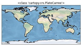
plt.axes(projection=ccrs.PlateCarree())
<GeoAxesSubplot:>

That was a little underwhelming, but we can see that the Axes created is indeed one of those GeoAxes[Subplot] instances.
One of the most useful methods that this class adds on top of the standard matplotlib Axes class is the coastlines method. With no arguments, it will add the Natural Earth 1:110,000,000 scale coastline data to the map.
plt.figure()
ax = plt.axes(projection=ccrs.PlateCarree())
ax.coastlines()
<cartopy.mpl.feature_artist.FeatureArtist at 0x7fc448ad7e80>
We could just as equally created a matplotlib subplot with one of the many approaches that exist. For example, the plt.subplots function could be used:
fig, ax = plt.subplots(subplot_kw={'projection': ccrs.PlateCarree()})
ax.coastlines()
<cartopy.mpl.feature_artist.FeatureArtist at 0x7fc453f68c10>

Projection classes have options we can use to customize the map
ccrs.PlateCarree?
Init signature: ccrs.PlateCarree(central_longitude=0.0, globe=None)
Docstring:
The abstract class which denotes cylindrical projections where we
want to allow x values to wrap around.
Init docstring:
Parameters
----------
proj4_params: iterable of key-value pairs
    The proj4 parameters required to define the
    desired CRS.  The parameters should not describe
    the desired elliptic model, instead create an
    appropriate Globe instance. The ``proj4_params``
    parameters will override any parameters that the
    Globe defines.
globe: :class:`~cartopy.crs.Globe` instance, optional
    If omitted, the default Globe instance will be created.
    See :class:`~cartopy.crs.Globe` for details.
File:           /srv/conda/envs/notebook/lib/python3.8/site-packages/cartopy/crs.py
Type:           ABCMeta
Subclasses:
ax = plt.axes(projection=ccrs.PlateCarree(central_longitude=180))
ax.coastlines()
<cartopy.mpl.feature_artist.FeatureArtist at 0x7fc453f99370>
Useful methods of a GeoAxes#
The cartopy.mpl.geoaxes.GeoAxes class adds a number of useful methods.
Let’s take a look at:
set_global - zoom the map out as much as possible
set_extent - zoom the map to the given bounding box
gridlines - add a graticule (and optionally labels) to the axes
coastlines - add Natural Earth coastlines to the axes
stock_img - add a low-resolution Natural Earth background image to the axes
imshow - add an image (numpy array) to the axes
add_geometries - add a collection of geometries (Shapely) to the axes
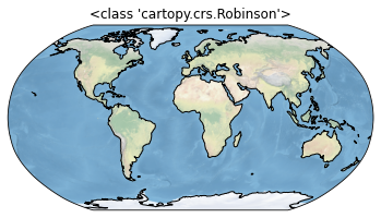
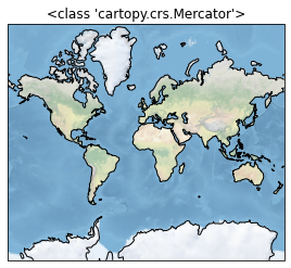
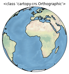
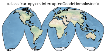
Some More Examples of Different Global Projections#
projections = [ccrs.PlateCarree(),
               ccrs.Robinson(),
               ccrs.Mercator(),
               ccrs.Orthographic(),
               ccrs.InterruptedGoodeHomolosine()
              ]


for proj in projections:
    plt.figure()
    ax = plt.axes(projection=proj)
    ax.stock_img()
    ax.coastlines()
    ax.set_title(f'{type(proj)}')
Regional Maps#
To create a regional map, we use the set_extent method of GeoAxis to limit the size of the region.
ax.set_extent?
Signature: ax.set_extent(extents, crs=None)
Docstring:
Set the extent (x0, x1, y0, y1) of the map in the given
coordinate system.

If no crs is given, the extents' coordinate system will be assumed
to be the Geodetic version of this axes' projection.

Parameters
----------
extents
    Tuple of floats representing the required extent (x0, x1, y0, y1).
File:      /srv/conda/envs/notebook/lib/python3.8/site-packages/cartopy/mpl/geoaxes.py
Type:      method
central_lon, central_lat = -10, 45
extent = [-40, 20, 30, 60]
ax = plt.axes(projection=ccrs.Orthographic(central_lon, central_lat))
ax.set_extent(extent)
ax.gridlines()
ax.coastlines(resolution='50m')
<cartopy.mpl.feature_artist.FeatureArtist at 0x7fc448d09160>
Adding Features to the Map#
To give our map more styles and details, we add cartopy.feature objects.
Many useful features are built in. These “default features” are at coarse (110m) resolution.
Name |
Description |
|---|---|
|
Country boundaries |
|
Coastline, including major islands |
|
Natural and artificial lakes |
|
Land polygons, including major islands |
|
Ocean polygons |
|
Single-line drainages, including lake centerlines |
|
(limited to the United States at this scale) |
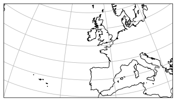
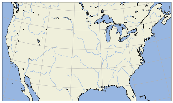
Below we illustrate these features in a customized map of North America.
import cartopy.feature as cfeature
import numpy as np

central_lat = 37.5
central_lon = -96
extent = [-120, -70, 24, 50.5]
central_lon = np.mean(extent[:2])
central_lat = np.mean(extent[2:])

plt.figure(figsize=(12, 6))
ax = plt.axes(projection=ccrs.AlbersEqualArea(central_lon, central_lat))
ax.set_extent(extent)

ax.add_feature(cartopy.feature.OCEAN)
ax.add_feature(cartopy.feature.LAND, edgecolor='black')
ax.add_feature(cartopy.feature.LAKES, edgecolor='black')
ax.add_feature(cartopy.feature.RIVERS)
ax.gridlines()
<cartopy.mpl.gridliner.Gridliner at 0x7fc448994970>
/srv/conda/envs/notebook/lib/python3.8/site-packages/cartopy/io/__init__.py:241: DownloadWarning: Downloading: https://naturalearth.s3.amazonaws.com/50m_physical/ne_50m_ocean.zip
  warnings.warn(f'Downloading: {url}', DownloadWarning)
/srv/conda/envs/notebook/lib/python3.8/site-packages/cartopy/io/__init__.py:241: DownloadWarning: Downloading: https://naturalearth.s3.amazonaws.com/50m_physical/ne_50m_lakes.zip
  warnings.warn(f'Downloading: {url}', DownloadWarning)
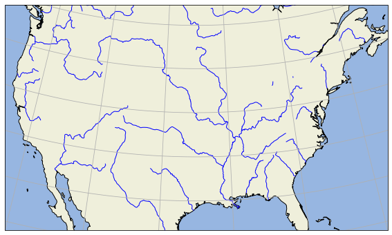
If we want higher-resolution features, Cartopy can automatically download and create them from the Natural Earth Data database or the GSHHS dataset database.
rivers_50m = cfeature.NaturalEarthFeature('physical', 'rivers_lake_centerlines', '50m')

plt.figure(figsize=(12, 6))
ax = plt.axes(projection=ccrs.AlbersEqualArea(central_lon, central_lat))
ax.set_extent(extent)

ax.add_feature(cartopy.feature.OCEAN)
ax.add_feature(cartopy.feature.LAND, edgecolor='black')
ax.add_feature(rivers_50m, facecolor='None', edgecolor='b')
ax.gridlines()
<cartopy.mpl.gridliner.Gridliner at 0x7fc448591880>
Adding Data to the Map#
Now that we know how to create a map, let’s add our data to it! That’s the whole point.
Because our map is a matplotlib axis, we can use all the familiar maptplotlib commands to make plots.
By default, the map extent will be adjusted to match the data. We can override this with the .set_global or .set_extent commands.
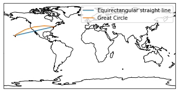
# create some test data
new_york = dict(lon=-74.0060, lat=40.7128)
honolulu = dict(lon=-157.8583, lat=21.3069)
lons = [new_york['lon'], honolulu['lon']]
lats = [new_york['lat'], honolulu['lat']]
Key point: the data also have to be transformed to the projection space.
This is done via the transform= keyword in the plotting method. The argument is another cartopy.crs object.
If you don’t specify a transform, Cartopy assume that the data is using the same projection as the underlying GeoAxis.
From the Cartopy Documentation
The core concept is that the projection of your axes is independent of the coordinate system your data is defined in. The
projectionargument is used when creating plots and determines the projection of the resulting plot (i.e. what the plot looks like). Thetransformargument to plotting functions tells Cartopy what coordinate system your data are defined in.
ax = plt.axes(projection=ccrs.PlateCarree())
ax.plot(lons, lats, label='Equirectangular straight line')
ax.plot(lons, lats, label='Great Circle', transform=ccrs.Geodetic())
ax.coastlines()
ax.legend()
ax.set_global()
Plotting 2D (Raster) Data#
The same principles apply to 2D data. Below we create some example data defined in regular lat / lon coordinates.
import numpy as np
lon = np.linspace(-80, 80, 25)
lat = np.linspace(30, 70, 25)
lon2d, lat2d = np.meshgrid(lon, lat)
data = np.cos(np.deg2rad(lat2d) * 4) + np.sin(np.deg2rad(lon2d) * 4)
plt.contourf(lon2d, lat2d, data)
<matplotlib.contour.QuadContourSet at 0x7fc4489320d0>
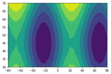
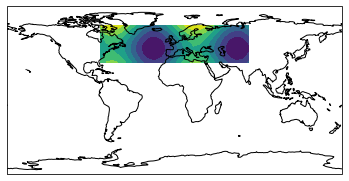
Now we create a PlateCarree projection and plot the data on it without any transform keyword.
This happens to work because PlateCarree is the simplest projection of lat / lon data.
ax = plt.axes(projection=ccrs.PlateCarree())
ax.set_global()
ax.coastlines()
ax.contourf(lon, lat, data)
<cartopy.mpl.contour.GeoContourSet at 0x7fc4485cd3d0>
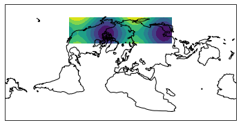
However, if we try the same thing with a different projection, we get the wrong result.
projection = ccrs.RotatedPole(pole_longitude=-177.5, pole_latitude=37.5)
ax = plt.axes(projection=projection)
ax.set_global()
ax.coastlines()
ax.contourf(lon, lat, data)
<cartopy.mpl.contour.GeoContourSet at 0x7fc448a8ad00>
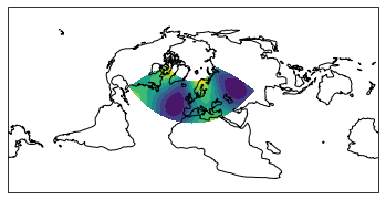
To fix this, we need to pass the correct transform argument to contourf:
projection = ccrs.RotatedPole(pole_longitude=-177.5, pole_latitude=37.5)
ax = plt.axes(projection=projection)
ax.set_global()
ax.coastlines()
ax.contourf(lon, lat, data, transform=ccrs.PlateCarree())
<cartopy.mpl.contour.GeoContourSet at 0x7fc44894d7f0>
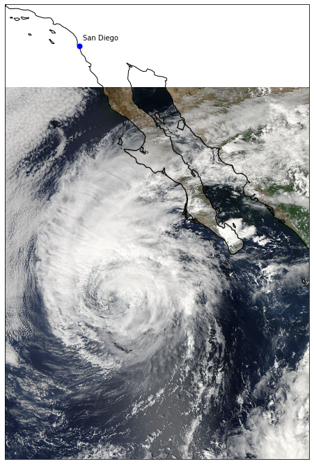
Showing Images#
We can plot a satellite image easily on a map if we know its extent
! wget https://lance-modis.eosdis.nasa.gov/imagery/gallery/2012270-0926/Miriam.A2012270.2050.2km.jpg
--2021-11-16 13:35:33--  https://lance-modis.eosdis.nasa.gov/imagery/gallery/2012270-0926/Miriam.A2012270.2050.2km.jpg
Resolving lance-modis.eosdis.nasa.gov (lance-modis.eosdis.nasa.gov)... 198.118.194.28, 2001:4d0:241a:40c0::28
Connecting to lance-modis.eosdis.nasa.gov (lance-modis.eosdis.nasa.gov)|198.118.194.28|:443... connected.
HTTP request sent, awaiting response... 301 Moved Permanently
Location: https://lance.modaps.eosdis.nasa.gov/imagery/gallery/2012270-0926/Miriam.A2012270.2050.2km.jpg [following]
--2021-11-16 13:35:33--  https://lance.modaps.eosdis.nasa.gov/imagery/gallery/2012270-0926/Miriam.A2012270.2050.2km.jpg
Resolving lance.modaps.eosdis.nasa.gov (lance.modaps.eosdis.nasa.gov)... 198.118.194.28, 2001:4d0:241a:40c0::28
Connecting to lance.modaps.eosdis.nasa.gov (lance.modaps.eosdis.nasa.gov)|198.118.194.28|:443... connected.
HTTP request sent, awaiting response... 200 OK
Length: 256220 (250K) [image/jpeg]
Saving to: ‘Miriam.A2012270.2050.2km.jpg’

Miriam.A2012270.205 100%[===================>] 250.21K  --.-KB/s    in 0.1s

2021-11-16 13:35:34 (1.94 MB/s) - ‘Miriam.A2012270.2050.2km.jpg’ saved [256220/256220]
fig = plt.figure(figsize=(8, 12))

# this is from the cartopy docs
fname = 'Miriam.A2012270.2050.2km.jpg'
img_extent = (-120.67660000000001, -106.32104523100001, 13.2301484511245, 30.766899999999502)
img = plt.imread(fname)

ax = plt.axes(projection=ccrs.PlateCarree())

# set a margin around the data
ax.set_xmargin(0.05)
ax.set_ymargin(0.10)

# add the image. Because this image was a tif, the "origin" of the image is in the
# upper left corner
ax.imshow(img, origin='upper', extent=img_extent, transform=ccrs.PlateCarree())
ax.coastlines(resolution='50m', color='black', linewidth=1)

# mark a known place to help us geo-locate ourselves
ax.plot(-117.1625, 32.715, 'bo', markersize=7, transform=ccrs.Geodetic())
ax.text(-117, 33, 'San Diego', transform=ccrs.Geodetic())
Text(-117, 33, 'San Diego')
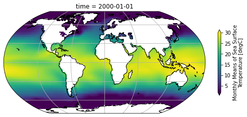
Xarray Integration#
Cartopy transforms can be passed to xarray! This creates a very quick path for creating professional looking maps from netCDF data.
import xarray as xr
url = 'http://www.esrl.noaa.gov/psd/thredds/dodsC/Datasets/noaa.ersst.v5/sst.mnmean.nc'
ds = xr.open_dataset(url, drop_variables=['time_bnds'])
ds
<xarray.Dataset>
Dimensions:  (lat: 89, lon: 180, time: 2014)
Coordinates:
  * lat      (lat) float32 88.0 86.0 84.0 82.0 80.0 ... -82.0 -84.0 -86.0 -88.0
  * lon      (lon) float32 0.0 2.0 4.0 6.0 8.0 ... 350.0 352.0 354.0 356.0 358.0
  * time     (time) datetime64[ns] 1854-01-01 1854-02-01 ... 2021-10-01
Data variables:
    sst      (time, lat, lon) float32 ...
Attributes: (12/38)
    climatology:                     Climatology is based on 1971-2000 SST, X...
    description:                     In situ data: ICOADS2.5 before 2007 and ...
    keywords_vocabulary:             NASA Global Change Master Directory (GCM...
    keywords:                        Earth Science > Oceans > Ocean Temperatu...
    instrument:                      Conventional thermometers
    source_comment:                  SSTs were observed by conventional therm...
    ...                              ...
    license:                         No constraints on data access or use
    comment:                         SSTs were observed by conventional therm...
    summary:                         ERSST.v5 is developed based on v4 after ...
    dataset_title:                   NOAA Extended Reconstructed SST V5
    data_modified:                   2021-11-07
DODS_EXTRA.Unlimited_Dimension: time- lat: 89
- lon: 180
- time: 2014
- lat(lat)float3288.0 86.0 84.0 ... -86.0 -88.0
- units :
- degrees_north
- long_name :
- Latitude
- actual_range :
- [ 88. -88.]
- standard_name :
- latitude
- axis :
- Y
- coordinate_defines :
- center
array([ 88., 86., 84., 82., 80., 78., 76., 74., 72., 70., 68., 66., 64., 62., 60., 58., 56., 54., 52., 50., 48., 46., 44., 42., 40., 38., 36., 34., 32., 30., 28., 26., 24., 22., 20., 18., 16., 14., 12., 10., 8., 6., 4., 2., 0., -2., -4., -6., -8., -10., -12., -14., -16., -18., -20., -22., -24., -26., -28., -30., -32., -34., -36., -38., -40., -42., -44., -46., -48., -50., -52., -54., -56., -58., -60., -62., -64., -66., -68., -70., -72., -74., -76., -78., -80., -82., -84., -86., -88.], dtype=float32) - lon(lon)float320.0 2.0 4.0 ... 354.0 356.0 358.0
- units :
- degrees_east
- long_name :
- Longitude
- actual_range :
- [ 0. 358.]
- standard_name :
- longitude
- axis :
- X
- coordinate_defines :
- center
array([ 0., 2., 4., 6., 8., 10., 12., 14., 16., 18., 20., 22., 24., 26., 28., 30., 32., 34., 36., 38., 40., 42., 44., 46., 48., 50., 52., 54., 56., 58., 60., 62., 64., 66., 68., 70., 72., 74., 76., 78., 80., 82., 84., 86., 88., 90., 92., 94., 96., 98., 100., 102., 104., 106., 108., 110., 112., 114., 116., 118., 120., 122., 124., 126., 128., 130., 132., 134., 136., 138., 140., 142., 144., 146., 148., 150., 152., 154., 156., 158., 160., 162., 164., 166., 168., 170., 172., 174., 176., 178., 180., 182., 184., 186., 188., 190., 192., 194., 196., 198., 200., 202., 204., 206., 208., 210., 212., 214., 216., 218., 220., 222., 224., 226., 228., 230., 232., 234., 236., 238., 240., 242., 244., 246., 248., 250., 252., 254., 256., 258., 260., 262., 264., 266., 268., 270., 272., 274., 276., 278., 280., 282., 284., 286., 288., 290., 292., 294., 296., 298., 300., 302., 304., 306., 308., 310., 312., 314., 316., 318., 320., 322., 324., 326., 328., 330., 332., 334., 336., 338., 340., 342., 344., 346., 348., 350., 352., 354., 356., 358.], dtype=float32) - time(time)datetime64[ns]1854-01-01 ... 2021-10-01
- long_name :
- Time
- delta_t :
- 0000-01-00 00:00:00
- avg_period :
- 0000-01-00 00:00:00
- prev_avg_period :
- 0000-00-07 00:00:00
- standard_name :
- time
- axis :
- T
- actual_range :
- [19723. 80992.]
- _ChunkSizes :
- 1
array(['1854-01-01T00:00:00.000000000', '1854-02-01T00:00:00.000000000',
       '1854-03-01T00:00:00.000000000', ..., '2021-08-01T00:00:00.000000000',
       '2021-09-01T00:00:00.000000000', '2021-10-01T00:00:00.000000000'],
      dtype='datetime64[ns]')
- sst(time, lat, lon)float32...
- long_name :
- Monthly Means of Sea Surface Temperature
- units :
- degC
- var_desc :
- Sea Surface Temperature
- level_desc :
- Surface
- statistic :
- Mean
- dataset :
- NOAA Extended Reconstructed SST V5
- parent_stat :
- Individual Values
- actual_range :
- [-1.8 42.32636]
- valid_range :
- [-1.8 45. ]
- _ChunkSizes :
- [ 1 89 180]
[32264280 values with dtype=float32]
- climatology :
- Climatology is based on 1971-2000 SST, Xue, Y., T. M. Smith, and R. W. Reynolds, 2003: Interdecadal changes of 30-yr SST normals during 1871.2000. Journal of Climate, 16, 1601-1612.
- description :
- In situ data: ICOADS2.5 before 2007 and NCEP in situ data from 2008 to present. Ice data: HadISST ice before 2010 and NCEP ice after 2010.
- keywords_vocabulary :
- NASA Global Change Master Directory (GCMD) Science Keywords
- keywords :
- Earth Science > Oceans > Ocean Temperature > Sea Surface Temperature >
- instrument :
- Conventional thermometers
- source_comment :
- SSTs were observed by conventional thermometers in Buckets (insulated or un-insulated canvas and wooded buckets) or Engine Room Intaker
- geospatial_lon_min :
- -1.0
- geospatial_lon_max :
- 359.0
- geospatial_laty_max :
- 89.0
- geospatial_laty_min :
- -89.0
- geospatial_lat_max :
- 89.0
- geospatial_lat_min :
- -89.0
- geospatial_lat_units :
- degrees_north
- geospatial_lon_units :
- degrees_east
- cdm_data_type :
- Grid
- project :
- NOAA Extended Reconstructed Sea Surface Temperature (ERSST)
- original_publisher_url :
- http://www.ncdc.noaa.gov
- References :
- https://www.ncdc.noaa.gov/data-access/marineocean-data/extended-reconstructed-sea-surface-temperature-ersst-v5 at NCEI and http://www.esrl.noaa.gov/psd/data/gridded/data.noaa.ersst.v5.html
- source :
- In situ data: ICOADS R3.0 before 2015, NCEP in situ GTS from 2016 to present, and Argo SST from 1999 to present. Ice data: HadISST2 ice before 2015, and NCEP ice after 2015
- title :
- NOAA ERSSTv5 (in situ only)
- history :
- created 07/2017 by PSD data using NCEI's ERSST V5 NetCDF values
- institution :
- This version written at NOAA/ESRL PSD: obtained from NOAA/NESDIS/National Centers for Environmental Information and time aggregated. Original Full Source: NOAA/NESDIS/NCEI/CCOG
- citation :
- Huang et al, 2017: Extended Reconstructed Sea Surface Temperatures Version 5 (ERSSTv5): Upgrades, Validations, and Intercomparisons. Journal of Climate, https://doi.org/10.1175/JCLI-D-16-0836.1
- platform :
- Ship and Buoy SSTs from ICOADS R3.0 and NCEP GTS
- standard_name_vocabulary :
- CF Standard Name Table (v40, 25 January 2017)
- processing_level :
- NOAA Level 4
- Conventions :
- CF-1.6, ACDD-1.3
- metadata_link :
- :metadata_link = https://doi.org/10.7289/V5T72FNM (original format)
- creator_name :
- Boyin Huang (original)
- date_created :
- 2017-06-30T12:18:00Z (original)
- product_version :
- Version 5
- creator_url_original :
- https://www.ncei.noaa.gov
- license :
- No constraints on data access or use
- comment :
- SSTs were observed by conventional thermometers in Buckets (insulated or un-insulated canvas and wooded buckets), Engine Room Intakers, or floats and drifters
- summary :
- ERSST.v5 is developed based on v4 after revisions of 8 parameters using updated data sets and advanced knowledge of ERSST analysis
- dataset_title :
- NOAA Extended Reconstructed SST V5
- data_modified :
- 2021-11-07
- DODS_EXTRA.Unlimited_Dimension :
- time
sst = ds.sst.sel(time='2000-01-01', method='nearest')
fig = plt.figure(figsize=(9,6))
ax = plt.axes(projection=ccrs.Robinson())
ax.coastlines()
ax.gridlines()
sst.plot(ax=ax, transform=ccrs.PlateCarree(),
         vmin=2, vmax=30, cbar_kwargs={'shrink': 0.4})
<cartopy.mpl.geocollection.GeoQuadMesh at 0x7fc42d31d580>
Doing More#
Browse the Cartopy Gallery to learn about all the different types of data and plotting methods available!