Working With Earth Science Model Output
Contents
Working With Earth Science Model Output#
In this lecture, we will discuss some fundamental aspects and techniques to work with the output of general circulation models (GCMs). These types of models are used in a variety of contexts in the Earth Science: From idealized experiments to understand meachanisms in the climate systems, to reanalyses and state estimates to synthesize past and current observations, to fully coupled representations of the earth system enabling forecasts of climate conditions under future scenarios.
What is a General Circulation Model?#
A GCM is a computer model that simulates the circulation of a fluid (e.g., the ocean or atmosphere). It is based on a set of partial differential equations, which describe the motion of a fluid in 3D space, and integrates these forward in time. Most fundamentally, these models use a discrete representation of the Navier-Stokes Equations but can include more equations to represent e.g., the thermodynamics, chemistry or biology of the coupled earth system. Depending on the goal these equations are forced with predetermined boundary conditions (e.g. an ocean only simulation is forced by observed atmospheric conditions) or the components of the earth system are coupled together and allowed to influence each other. A ‘climate model’ is often the latter case which is forced by e.g. different scenarios of greenhouse gas emissions. This enables predictions of how the coupled system will evolve in the future.
The globe divided into boxes#
Since there is no analytical solution to the full Navier-Stokes equation, modern GCMs solve them using numerical methods. They use a discretized version of the equations, which approximates them within a finite volume, or grid-cell. Each GCM splits the ocean or atmosphere into many cells, both in the horizontal and vertical.
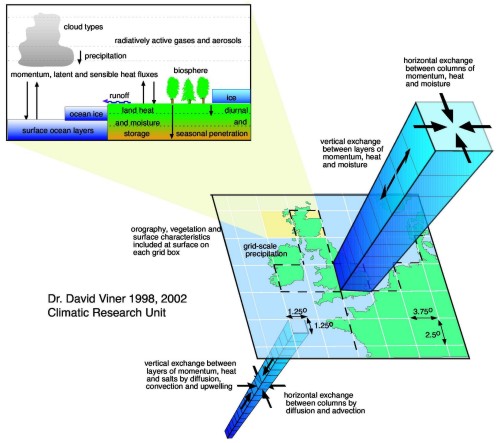
Source: www.ipcc-data.org
It is numerically favorable to shift (or ‘stagger’) the grid points where the model calculates the velocity with regard to the grid point where tracer values (temperature, salinity, or others) are calculated. There are several different ways to shift these points, commonly referred to as Arakawa grids. Most modern ocean models use a C-Grid. Thus, this lecture will focus on this particular grid configuration. In the C-grid, the zonal velocity \(u\) is located on the right side (or east face) of the tracer location and the meridional velocity \(v\) is located on the upper side (or north face). Similarly, the vertical velocity \(w\) is shifted with depth, but horizontally (when looking at it from straight above), it is on the tracer location.

Source: xgcm.readthedocs.io
Most GCMs use a curvilinear grid to avoid infinitely small grid cells at the North Pole. Some examples of curvilinear grids are a tripolar grid (the Arctic region is defined by two poles, placed over landmasses)
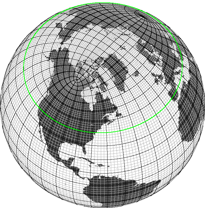
Source: GEOMAR
or a cubed-sphere grid or a lat-lon cap (different versions of connected patches of curvilinear grids).
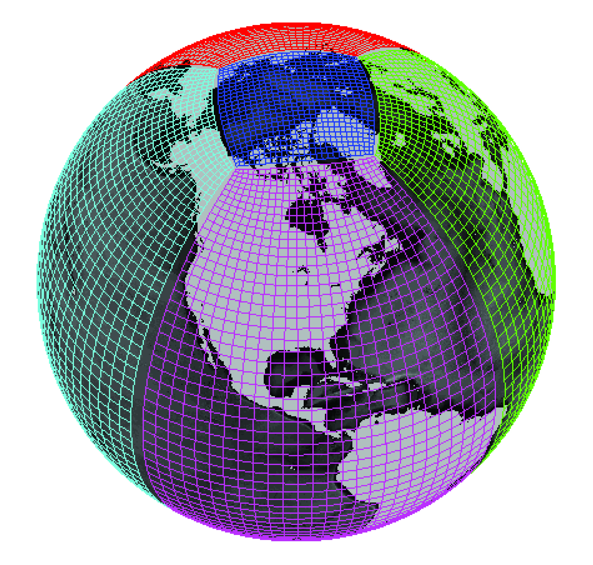
Credit: Gael Forget. More information about the simulation and grid available at https://doi.org/10.5194/gmd-8-3071-2015.
In most ocean models, due to these ‘warped’ coordinate systems, the boxes described are not perfectly rectangular cuboids. To accurately represent the volume of the cell, we require so-called grid metrics - the distances, cell areas, and volume to calculate operators like e.g., divergence.
If you want to compare models with different grids it can sometimes be necessary to regrid your output. However, some calculations should be performed on the native model grid for maximum accuracy. We will discuss these different cases below.
Grid resolution#
Discretizing the equations has consequences:
In order to get a realistic representation of the global circulation, the size of grid cells needs to be chosen so that all relevant processes are resolved. In reality, this usually requires too much computing power for global models and so processes that are too small to be explicitly resolved, like mesoscale eddies or vertical mixing, need to be carefully parameterized since they influence the large scale circulation. The following video illustrates the representation of mesoscale eddies in global models of different grid resolution. It shows the surface nutrient fields of three coupled climate models (produced by NOAA/GFDL) around the Antarctic Peninsula with increasing ocean resolution from left to right.
Nominal model resolution from left to right: 1 degree (CM2.1deg), 0.25 degree (CM2.5) and 0.1 degree (CM2.6). The left ocean model employs a parametrization for both the advective and diffusive effects of mesoscale eddies, while the middle and right model do not.
Goals of this section#
The aim of this book section is to teach you the basic techniques to work with output of GCM data of various ‘flavors’.
We will learn how to compare different climate model simulations from the CMIP6 project with each other.
We will learn how to
regridhigh-resolution model fields in order to compare them to observations.
We will learn how to use xgcm in order to deal with computations on the raw model grid for maximum accuracy.