Assignment: Numpy and Matplotlib
Contents
Assignment: Numpy and Matplotlib#
The goal of this assignment is to gain comfort creating, visualizating, and computing with numpy array. By the end of the assignment, you should feel comfortable:
Learning Goals
Creating new arrays using
linspaceandarangeComputing basic formulas with numpy arrays
Loading data from
.npyfilesPerforming reductions (e.g.
mean,stdon numpy arrays)Making 1D line plots
Making scatterplots
Annotating plots with titles and axes
1 Creating and Manipulating Arrays#
First import numpy and matplotlib
1.1. Create two 2D arrays representing coordinates x, y on the cartesian plan#
Both should cover the range (-2, 2) and have 100 points in each direction
1.2. Visualize each 2D array using pcolormesh#
Use the correct coordiantes for the x and y axes.
1.3 From your cartesian coordinates, create polar coordinates \(r\) and \(\varphi\)#
Refer to the wikipedia page for the conversion formula. You will need to use numpy’s arctan2 function. Read its documentation.
1.4. Visualize \(r\) and \(\varphi\) on the 2D \(x\) / \(y\) plane using pcolormesh#
1.5 Caclulate the quanity \(f = \cos^2(4r) + \sin^2(4\varphi)\)#
And plot it on the x\( / \)y$ plane
1.6 Plot the mean of f with respect to the x axis#
as a function of y
1.7 Plot the mean of f with respect to the y axis#
as a function of x
1.8 Plot the mean of \(f\) with respect to \(\phi\) as a function of \(r\)#
This is hard. You will need to define a discrete range of \(r\) values and then figure out how to average \(f\) within the bins defined by your \(r\) grid. There are many different ways to accomplish this.
Part 2: Analyze ARGO Data#
In this problem, we use real data from ocean profiling floats. ARGO floats are autonomous robotic instruments that collect Temperature, Salinity, and Pressure data from the ocean. ARGO floats collect one “profile” (a set of messurements at different depths or “levels”).
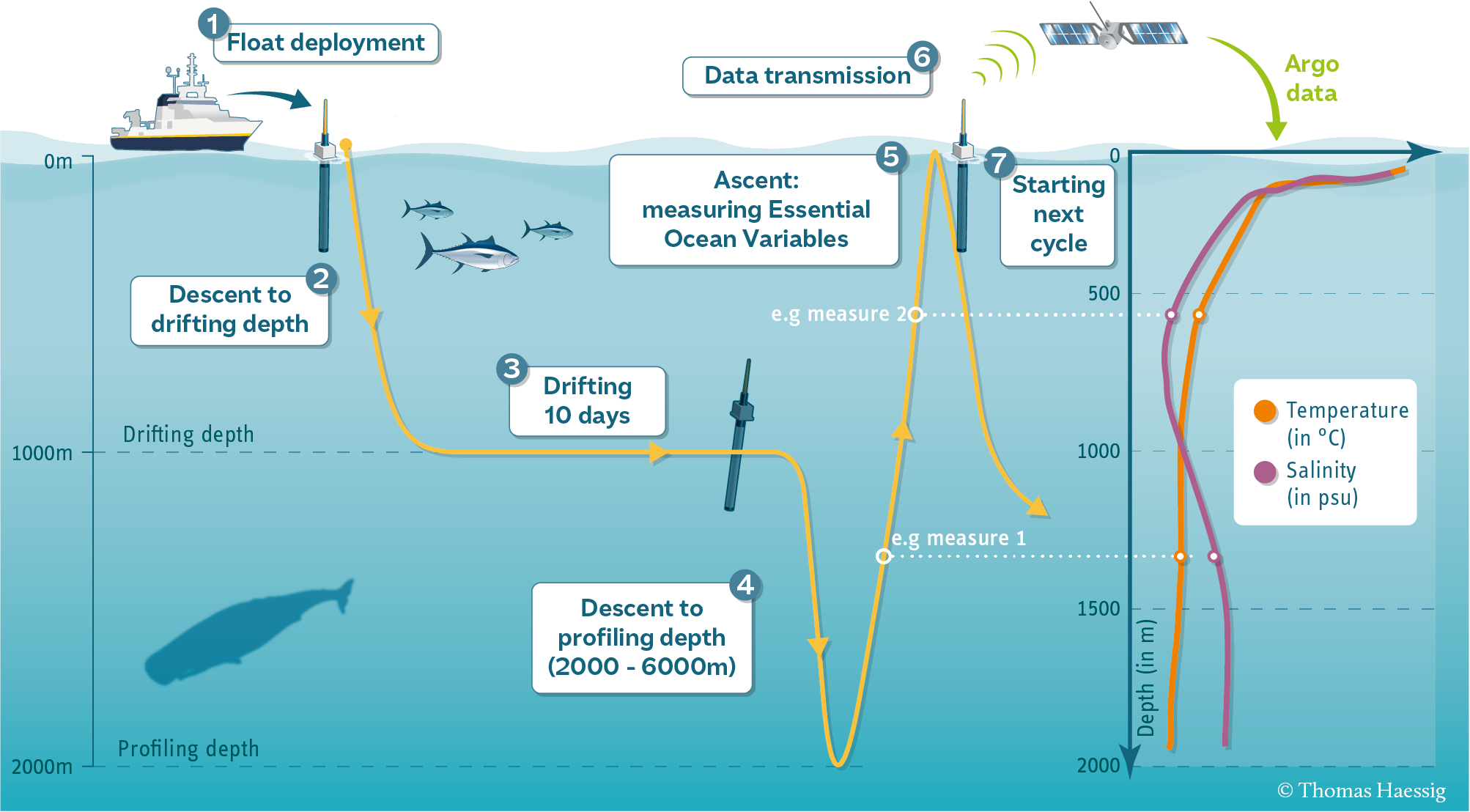
Each profile has a single latitude, longitude, and date associated with it, in addition to many different levels.
Let’s start by using pooch to download the data files we need for this exercise.
The following code will give you a list of .npy files that you can open in the next step.
import pooch
url = "https://www.ldeo.columbia.edu/~rpa/float_data_4901412.zip"
files = pooch.retrieve(url, processor=pooch.Unzip(), known_hash="2a703c720302c682f1662181d329c9f22f9f10e1539dc2d6082160a469165009")
files
2.1 Load each data file as a numpy array.#
You can use whatever names you want for your arrays, but I recommend
T: temperature
S: salinity
P: pressure
date: date
lat: latitude
lon: longitude
level: depth level
Note: you have to actually look at the file name (the items in files) to know which files corresponds to which variable.
2.3 Make a plot for each column of data in T, S and P (three plots).#
The vertical scale should be the levels data. Each plot should have a line for each column of data. It will look messy.
2.4 Compute the mean and standard deviation of each of T, S and P at each depth in level.#
2.5 Now make three similar plot, but show only the mean T, S and P at each depth. Show error bars on each plot using the standard deviations.#
2.6 Account For Missing Data#
The profiles contain many missing values. These are indicated by the special “Not a Number” value, or np.nan.
When you take the mean or standard deviation of data with NaNs in it, the entire result becomes NaN. Instead, if you use the special functions np.nanmean and np.nanstd, you tell NumPy to ignore the NaNs.
Recalculate the means and standard deviations as in the previous sections using these functions and plot the results.
2.7 Create a scatter plot of the lon, lat positions of the ARGO float.#
Use the plt.scatter function.