Pandas: Groupby#

groupby is an amazingly powerful function in pandas. But it is also complicated to use and understand. The point of this lesson is to make you feel confident in using groupby and its cousins, resample and rolling.

These notes are loosely based on the Pandas GroupBy Documentation.

The “split/apply/combine” concept was first introduced in a paper by Hadley Wickham: https://www.jstatsoft.org/article/view/v040i01.

Imports:

import numpy as np
from matplotlib import pyplot as plt
plt.rcParams['figure.figsize'] = (12,7)
%matplotlib inline
import pandas as pd

First we read the Earthquake data from our previous assignment:

df = pd.read_csv('http://www.ldeo.columbia.edu/~rpa/usgs_earthquakes_2014.csv', parse_dates=['time'], index_col='id')
df['country'] = df.place.str.split(', ').str[-1]
df_small = df[df.mag<4]
df = df[df.mag>4]
df.head()

	time	latitude	longitude	depth	mag	magType	nst	gap	dmin	rms	net	updated	place	type	country
id
usc000mqlp	2014-01-31 23:08:03.660	-4.9758	153.9466	110.18	4.2	mb	NaN	98.0	1.940	0.61	us	2014-04-08T01:43:19.000Z	115km ESE of Taron, Papua New Guinea	earthquake	Papua New Guinea
usc000mqln	2014-01-31 22:54:32.970	-28.1775	-177.9058	95.84	4.3	mb	NaN	104.0	1.063	1.14	us	2014-04-08T01:43:19.000Z	120km N of Raoul Island, New Zealand	earthquake	New Zealand
usc000mqls	2014-01-31 22:49:49.740	-23.1192	179.1174	528.34	4.4	mb	NaN	80.0	5.439	0.95	us	2014-04-08T01:43:19.000Z	South of the Fiji Islands	earthquake	South of the Fiji Islands
usc000mf1x	2014-01-31 22:19:44.330	51.1569	-178.0910	37.50	4.2	mb	NaN	NaN	NaN	0.83	us	2014-04-08T01:43:19.000Z	72km E of Amatignak Island, Alaska	earthquake	Alaska
usc000mqlm	2014-01-31 21:56:44.320	-4.8800	153.8434	112.66	4.3	mb	NaN	199.0	1.808	0.79	us	2014-04-08T01:43:19.000Z	100km ESE of Taron, Papua New Guinea	earthquake	Papua New Guinea

An Example#

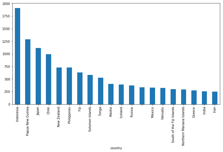
This is an example of a “one-liner” that you can accomplish with groupby.

df.groupby('country').mag.count().nlargest(20).plot(kind='bar', figsize=(12,6))

<matplotlib.axes._subplots.AxesSubplot at 0x112e20780>

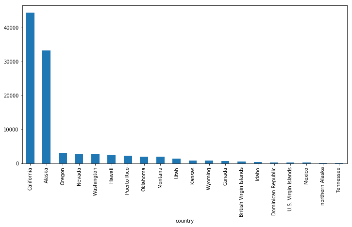
df_small.groupby('country').mag.count().nlargest(20).plot(kind='bar', figsize=(12,6))

<matplotlib.axes._subplots.AxesSubplot at 0x112b42d68>

What Happened?#

Let’s break apart this operation a bit. The workflow with groubpy can be divided into three general steps:

Split: Partition the data into different groups based on some criterion.
Apply: Do some caclulation within each group. Different types of “apply” steps might be
Aggregation: Get the mean or max within the group.
Transformation: Normalize all the values within a group
Filtration: Eliminate some groups based on a criterion.
Combine: Put the results back together into a single object.

split-apply-combine

The `groupby` method#

Both Series and DataFrame objects have a groupby method. It accepts a variety of arguments, but the simplest way to think about it is that you pass another series, whose unique values are used to split the original object into different groups.

via https://medium.com/analytics-vidhya/split-apply-combine-strategy-for-data-mining-4fd6e2a0cc99

df.groupby(df.country)

<pandas.core.groupby.DataFrameGroupBy object at 0x10626f358>

There is a shortcut for doing this with dataframes: you just pass the column name:

df.groupby('country')

<pandas.core.groupby.DataFrameGroupBy object at 0x10626f208>

The `GroubBy` object#

When we call, groupby we get back a GroupBy object:

gb = df.groupby('country')
gb

<pandas.core.groupby.DataFrameGroupBy object at 0x1131bcf60>

The length tells us how many groups were found:

len(gb)

All of the groups are available as a dictionary via the .groups attribute:

groups = gb.groups
len(groups)

list(groups.keys())

['',
 'Afghanistan',
 'Alaska',
 'Albania',
 'Algeria',
 'American Samoa',
 'Angola',
 'Anguilla',
 'Antarctica',
 'Argentina',
 'Arizona',
 'Aruba',
 'Ascension Island region',
 'Australia',
 'Azerbaijan',
 'Azores Islands region',
 'Azores-Cape St. Vincent Ridge',
 'Balleny Islands region',
 'Banda Sea',
 'Bangladesh',
 'Barbados',
 'Barbuda',
 'Bay of Bengal',
 'Bermuda',
 'Bhutan',
 'Bolivia',
 'Bosnia and Herzegovina',
 'Bouvet Island',
 'Bouvet Island region',
 'Brazil',
 'British Indian Ocean Territory',
 'British Virgin Islands',
 'Burma',
 'Burundi',
 'California',
 'Canada',
 'Cape Verde',
 'Carlsberg Ridge',
 'Cayman Islands',
 'Celebes Sea',
 'Central East Pacific Rise',
 'Central Mid-Atlantic Ridge',
 'Chagos Archipelago region',
 'Chile',
 'China',
 'Christmas Island',
 'Colombia',
 'Comoros',
 'Cook Islands',
 'Costa Rica',
 'Crozet Islands region',
 'Cuba',
 'Cyprus',
 'Davis Strait',
 'Democratic Republic of the Congo',
 'Djibouti',
 'Dominica',
 'Dominican Republic',
 'Drake Passage',
 'East Timor',
 'East of Severnaya Zemlya',
 'East of the Kuril Islands',
 'East of the North Island of New Zealand',
 'East of the Philippine Islands',
 'East of the South Sandwich Islands',
 'Easter Island region',
 'Eastern Greenland',
 'Ecuador',
 'Ecuador region',
 'Egypt',
 'El Salvador',
 'Eritrea',
 'Ethiopia',
 'Falkland Islands region',
 'Federated States of Micronesia region',
 'Fiji',
 'Fiji region',
 'France',
 'French Polynesia',
 'French Southern Territories',
 'Galapagos Triple Junction region',
 'Georgia',
 'Greece',
 'Greenland',
 'Greenland Sea',
 'Guadeloupe',
 'Guam',
 'Guatemala',
 'Gulf of Alaska',
 'Haiti',
 'Hawaii',
 'Honduras',
 'Iceland',
 'Idaho',
 'India',
 'India region',
 'Indian Ocean Triple Junction',
 'Indonesia',
 'Iran',
 'Iraq',
 'Italy',
 'Japan',
 'Japan region',
 'Jordan',
 'Kansas',
 'Kazakhstan',
 'Kermadec Islands region',
 'Kosovo',
 'Kuril Islands',
 'Kyrgyzstan',
 'Labrador Sea',
 'Laptev Sea',
 'Macedonia',
 'Macquarie Island region',
 'Malawi',
 'Malaysia',
 'Mariana Islands region',
 'Martinique',
 'Mauritania',
 'Mauritius',
 'Mauritius - Reunion region',
 'Mexico',
 'Micronesia',
 'Mid-Indian Ridge',
 'Molucca Sea',
 'Mongolia',
 'Montana',
 'Montenegro',
 'Morocco',
 'Mozambique',
 'Mozambique Channel',
 'Nepal',
 'New Caledonia',
 'New Mexico',
 'New Zealand',
 'Nicaragua',
 'Niue',
 'North Atlantic Ocean',
 'North Indian Ocean',
 'North Korea',
 'North of Ascension Island',
 'North of Franz Josef Land',
 'North of New Zealand',
 'North of Severnaya Zemlya',
 'North of Svalbard',
 'Northern East Pacific Rise',
 'Northern Mariana Islands',
 'Northern Mid-Atlantic Ridge',
 'Northwest of Australia',
 'Norway',
 'Norwegian Sea',
 'Off the coast of Central America',
 'Off the coast of Ecuador',
 'Off the coast of Oregon',
 'Off the east coast of the North Island of New Zealand',
 'Off the south coast of Australia',
 'Off the west coast of northern Sumatra',
 'Oklahoma',
 'Oman',
 'Oregon',
 'Owen Fracture Zone region',
 'Pacific-Antarctic Ridge',
 'Pakistan',
 'Palau',
 'Palau region',
 'Panama',
 'Papua New Guinea',
 'Peru',
 'Peru-Ecuador border region',
 'Philippine Islands region',
 'Philippines',
 'Poland',
 'Portugal',
 'Portugal region',
 'Prince Edward Islands',
 'Prince Edward Islands region',
 'Puerto Rico',
 'Republic of the Congo',
 'Reykjanes Ridge',
 'Romania',
 'Russia',
 'Russia region',
 'Saint Helena',
 'Saint Lucia',
 'Saint Vincent and the Grenadines',
 'Samoa',
 'Santa Cruz Islands region',
 'Saudi Arabia',
 'Scotia Sea',
 'Sea of Okhotsk',
 'Serbia',
 'Slovenia',
 'Socotra region',
 'Solomon Islands',
 'Somalia',
 'South Africa',
 'South Atlantic Ocean',
 'South Carolina',
 'South Georgia Island region',
 'South Georgia and the South Sandwich Islands',
 'South Indian Ocean',
 'South Napa Earthquake',
 'South Sandwich Islands',
 'South Sandwich Islands region',
 'South Shetland Islands',
 'South Sudan',
 'South of Africa',
 'South of Australia',
 'South of Panama',
 'South of Tasmania',
 'South of Tonga',
 'South of the Fiji Islands',
 'South of the Kermadec Islands',
 'South of the Mariana Islands',
 'Southeast Indian Ridge',
 'Southeast central Pacific Ocean',
 'Southeast of Easter Island',
 'Southern East Pacific Rise',
 'Southern Mid-Atlantic Ridge',
 'Southern Pacific Ocean',
 'Southwest Indian Ridge',
 'Southwest of Africa',
 'Southwest of Australia',
 'Southwestern Atlantic Ocean',
 'Spain',
 'Sudan',
 'Svalbard and Jan Mayen',
 'Sweden',
 'Syria',
 'Taiwan',
 'Tajikistan',
 'Tanzania',
 'Thailand',
 'Tonga',
 'Tonga region',
 'Trinidad and Tobago',
 'Tristan da Cunha region',
 'Turkey',
 'Turkmenistan',
 'Uganda',
 'Ukraine',
 'United Kingdom',
 'Utah',
 'Uzbekistan',
 'Vanuatu',
 'Vanuatu region',
 'Venezuela',
 'Vietnam',
 'Wallis and Futuna',
 'West Chile Rise',
 'West of Australia',
 'West of Macquarie Island',
 'West of Vancouver Island',
 'West of the Galapagos Islands',
 'Western Australia',
 'Western Indian-Antarctic Ridge',
 'Yemen',
 'Zambia',
 'north of Ascension Island',
 'northern Mid-Atlantic Ridge',
 'south of Panama',
 'western Xizang']

Iterating and selecting groups#

You can loop through the groups if you want.

for key, group in gb:
    display(group.head())
    print(f'The key is "{key}"')
    break

	time	latitude	longitude	depth	mag	magType	nst	gap	dmin	rms	net	updated	place	type
id
usc000mkc8	2014-01-25 16:10:38.760	-55.2925	-27.0527	10.00	4.1	mb	NaN	97.0	5.553	0.35	us	2014-03-27T18:15:40.000Z	156km N of Visokoi Island,	earthquake
usc000mkc7	2014-01-25 09:43:23.230	-55.9434	-27.6772	103.48	4.3	mb	NaN	87.0	5.324	0.62	us	2014-03-27T18:15:40.000Z	89km NNW of Visokoi Island,	earthquake
usc000mh0c	2014-01-19 15:42:45.510	-56.9656	-26.7803	120.25	4.6	mb	NaN	151.0	6.120	0.39	us	2014-03-22T00:05:23.000Z	39km SE of Visokoi Island,	earthquake
usb000m7f2	2014-01-10 13:50:38.730	-56.0110	-26.1186	10.00	4.2	mb	NaN	106.0	6.192	0.71	us	2014-03-15T03:38:58.000Z	101km NE of Visokoi Island,	earthquake
usb000m78v	2014-01-07 06:51:09.160	-56.9651	-26.6696	124.37	4.3	mb	NaN	109.0	6.176	0.59	us	2014-03-07T00:26:01.000Z	43km SE of Visokoi Island,	earthquake

The key is ""

And you can get a specific group by key.

gb.get_group('Chile').head()

	time	latitude	longitude	depth	mag	magType	nst	gap	dmin	rms	net	updated	place	type	country
id
usc000mqlq	2014-01-31 20:00:16.000	-33.6550	-71.9810	25.10	4.5	mb	NaN	NaN	NaN	1.63	us	2014-04-08T01:43:19.000Z	34km WSW of San Antonio, Chile	earthquake	Chile
usc000mql6	2014-01-31 13:48:23.000	-18.0690	-69.6630	149.10	4.3	mb	NaN	NaN	NaN	1.77	us	2014-04-08T01:43:18.000Z	17km NW of Putre, Chile	earthquake	Chile
usc000mqk8	2014-01-30 14:20:56.560	-19.6118	-70.9487	15.16	4.1	mb	NaN	159.0	1.227	1.34	us	2014-04-08T01:43:17.000Z	107km NW of Iquique, Chile	earthquake	Chile
usc000mdi2	2014-01-30 10:02:14.000	-32.1180	-71.7860	25.70	4.5	mwr	NaN	NaN	NaN	1.10	us	2015-01-30T21:28:21.955Z	64km NW of La Ligua, Chile	earthquake	Chile
usc000mqeh	2014-01-29 18:58:23.000	-18.6610	-69.6440	123.10	4.8	mb	NaN	NaN	NaN	1.52	us	2014-04-08T01:43:16.000Z	51km S of Putre, Chile	earthquake	Chile

Aggregation#

Now that we know how to create a GroupBy object, let’s learn how to do aggregation on it.

One way us to use the .aggregate method, which accepts another function as its argument. The result is automatically combined into a new dataframe with the group key as the index.

gb.aggregate(np.max).head()

	time	latitude	longitude	depth	mag	magType	nst	gap	dmin	rms	net	updated	place	type
country
	2014-12-31 14:49:19.200	-37.5219	78.9418	248.18	6.9	mww	NaN	195.0	28.762	1.47	us	2015-03-17T02:38:27.040Z	99km NW of Visokoi Island,	earthquake
Afghanistan	2014-12-27 06:37:50.010	37.0112	71.6062	248.39	5.6	mww	NaN	172.0	3.505	1.55	us	2015-06-22T20:12:10.712Z	8km SE of Ashkasham, Afghanistan	earthquake
Alaska	2014-12-30 21:22:21.580	67.9858	179.9288	266.61	7.9	mww	152.0	338.0	7.712	2.15	us	2015-05-30T05:34:08.822Z	9km WSW of Little Sitkin Island, Alaska	earthquake
Albania	2014-05-20 04:43:25.500	41.5297	20.2804	28.26	5.0	mwr	NaN	69.0	1.299	1.34	us	2015-01-30T15:28:03.533Z	6km NE of Durres, Albania	earthquake
Algeria	2014-12-26 17:55:18.140	36.9391	5.6063	21.40	5.5	mww	NaN	174.0	3.250	1.45	us	2015-03-17T02:37:18.040Z	5km SSW of Bougara, Algeria	earthquake

By default, the operation is applied to every column. That’s usually not what we want. We can use both . or [] syntax to select a specific column to operate on. Then we get back a series.

gb.mag.aggregate(np.max).head()

country
               6.9
Afghanistan    5.6
Alaska         7.9
Albania        5.0
Algeria        5.5
Name: mag, dtype: float64

gb.mag.aggregate(np.max).nlargest(10)

country
Chile                         8.2
Alaska                        7.9
Solomon Islands               7.6
Papua New Guinea              7.5
El Salvador                   7.3
Mexico                        7.2
Fiji                          7.1
Indonesia                     7.1
Southern East Pacific Rise    7.0
                              6.9
Name: mag, dtype: float64

There are shortcuts for common aggregation functions:

gb.mag.max().nlargest(10)

country
Chile                         8.2
Alaska                        7.9
Solomon Islands               7.6
Papua New Guinea              7.5
El Salvador                   7.3
Mexico                        7.2
Fiji                          7.1
Indonesia                     7.1
Southern East Pacific Rise    7.0
                              6.9
Name: mag, dtype: float64

gb.mag.min().nsmallest(10)

country
Mexico         4.01
Oregon         4.02
California     4.04
               4.10
Afghanistan    4.10
Alaska         4.10
Albania        4.10
Algeria        4.10
Angola         4.10
Antarctica     4.10
Name: mag, dtype: float64

gb.mag.mean().nlargest(10)

country
South Napa Earthquake          6.020000
Bouvet Island region           5.750000
South Georgia Island region    5.450000
Barbados                       5.400000
New Mexico                     5.300000
Easter Island region           5.162500
Malawi                         5.100000
Drake Passage                  5.033333
North Korea                    5.000000
Saint Lucia                    5.000000
Name: mag, dtype: float64

gb.mag.std().nlargest(10)

country
Barbados                              1.555635
Bouvet Island region                  1.484924
Puerto Rico                           0.957601
Off the coast of Ecuador              0.848528
Palau region                          0.777817
East of the South Sandwich Islands    0.606495
Southern East Pacific Rise            0.604508
South Indian Ocean                    0.602194
Prince Edward Islands region          0.595259
Panama                                0.591322
Name: mag, dtype: float64

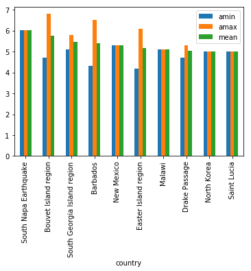
We can also apply multiple functions at once:

gb.mag.aggregate([np.min, np.max, np.mean]).head()

	amin	amax	mean
country
	4.1	6.9	4.582544
Afghanistan	4.1	5.6	4.410656
Alaska	4.1	7.9	4.515025
Albania	4.1	5.0	4.391667
Algeria	4.1	5.5	4.583333

gb.mag.aggregate([np.min, np.max, np.mean]).nlargest(10, 'mean').plot(kind='bar')

<matplotlib.axes._subplots.AxesSubplot at 0x112a09e80>

Transformation#

The key difference between aggregation and transformation is that aggregation returns a smaller object than the original, indexed by the group keys, while transformation returns an object with the same index (and same size) as the original object. Groupby + transformation is used when applying an operation that requires information about the whole group.

In this example, we standardize the earthquakes in each country so that the distribution has zero mean and unit variance. We do this by first defining a function called standardize and then passing it to the transform method.

I admit that I don’t know why you would want to do this. transform makes more sense to me in the context of time grouping operation. See below for another example.

def standardize(x):
    return (x - x.mean())/x.std()

mag_standardized_by_country = gb.mag.transform(standardize)
mag_standardized_by_country.head()

id
usc000mqlp   -0.915774
usc000mqln   -0.675696
usc000mqls   -0.282385
usc000mf1x   -0.684915
usc000mqlm   -0.666807
Name: mag, dtype: float64

Time Grouping#

We already saw how pandas has a strong built-in understanding of time. This capability is even more powerful in the context of groupby. With datasets indexed by a pandas DateTimeIndex, we can easily group and resample the data using common time units.

To get started, let’s load the timeseries data we already explored in past lessons.

import urllib
import pandas as pd

header_url = 'ftp://ftp.ncdc.noaa.gov/pub/data/uscrn/products/daily01/HEADERS.txt'
with urllib.request.urlopen(header_url) as response:
    data = response.read().decode('utf-8')
lines = data.split('\n')
headers = lines[1].split(' ')

ftp_base = 'ftp://ftp.ncdc.noaa.gov/pub/data/uscrn/products/daily01/'
dframes = []
for year in range(2016, 2019):
    data_url = f'{year}/CRND0103-{year}-NY_Millbrook_3_W.txt'               
    df = pd.read_csv(ftp_base + data_url, parse_dates=[1],
                     names=headers, header=None, sep='\s+',
                     na_values=[-9999.0, -99.0])
    dframes.append(df)

df = pd.concat(dframes)
df = df.set_index('LST_DATE')

df.head()

	WBANNO	CRX_VN	LONGITUDE	LATITUDE	T_DAILY_MAX	T_DAILY_MIN	T_DAILY_MEAN	T_DAILY_AVG	P_DAILY_CALC	SOLARAD_DAILY	...	SOIL_MOISTURE_10_DAILY	SOIL_MOISTURE_20_DAILY	SOIL_MOISTURE_50_DAILY	SOIL_MOISTURE_100_DAILY	SOIL_TEMP_5_DAILY	SOIL_TEMP_10_DAILY	SOIL_TEMP_20_DAILY	SOIL_TEMP_50_DAILY	SOIL_TEMP_100_DAILY
LST_DATE
2016-01-01	64756	2.422	-73.74	41.79	3.4	-0.5	1.5	1.3	0.0	1.69	...	0.233	0.204	0.155	0.147	4.2	4.4	5.1	6.0	7.6	NaN
2016-01-02	64756	2.422	-73.74	41.79	2.9	-3.6	-0.4	-0.3	0.0	6.25	...	0.227	0.199	0.152	0.144	2.8	3.1	4.2	5.7	7.4	NaN
2016-01-03	64756	2.422	-73.74	41.79	5.1	-1.8	1.6	1.1	0.0	5.69	...	0.223	0.196	0.151	0.141	2.6	2.8	3.8	5.2	7.2	NaN
2016-01-04	64756	2.422	-73.74	41.79	0.5	-14.4	-6.9	-7.5	0.0	9.17	...	0.220	0.194	0.148	0.139	1.7	2.1	3.4	4.9	6.9	NaN
2016-01-05	64756	2.422	-73.74	41.79	-5.2	-15.5	-10.3	-11.7	0.0	9.34	...	0.213	0.191	0.148	0.138	0.4	0.9	2.4	4.3	6.6	NaN

5 rows × 28 columns

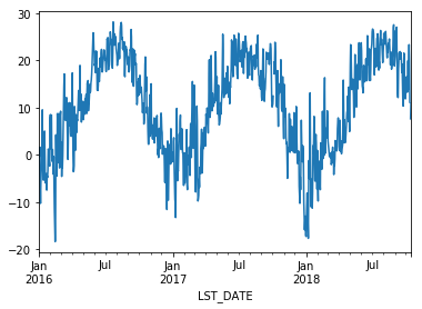
This timeseries has daily resolution, and the daily plots are somewhat noisy.

df.T_DAILY_MEAN.plot()

<matplotlib.axes._subplots.AxesSubplot at 0x112f05b00>

A common way to analyze such data in climate science is to create a “climatology,” which contains the average values in each month or day of the year. We can do this easily with groupby. Recall that df.index is a pandas DateTimeIndex object.

monthly_climatology = df.groupby(df.index.month).mean()
monthly_climatology

	WBANNO	CRX_VN	LONGITUDE	LATITUDE	T_DAILY_MAX	T_DAILY_MIN	T_DAILY_MEAN	T_DAILY_AVG	P_DAILY_CALC	SOLARAD_DAILY	...	SOIL_MOISTURE_10_DAILY	SOIL_MOISTURE_20_DAILY	SOIL_MOISTURE_50_DAILY	SOIL_MOISTURE_100_DAILY	SOIL_TEMP_5_DAILY	SOIL_TEMP_10_DAILY	SOIL_TEMP_20_DAILY	SOIL_TEMP_50_DAILY	SOIL_TEMP_100_DAILY
LST_DATE
1	64756	2.488667	-73.74	41.79	2.924731	-7.120430	-2.100000	-1.905376	2.480645	5.811613	...	0.240292	0.199547	0.150376	0.162533	0.168817	0.232258	0.788172	1.749462	3.394624	NaN
2	64756	2.487882	-73.74	41.79	6.431765	-5.015294	0.712941	1.022353	4.080000	8.495176	...	0.244286	0.203089	0.154306	0.165506	1.217647	1.183529	1.280000	1.602353	2.460000	NaN
3	64756	2.488667	-73.74	41.79	7.953763	-3.035484	2.455914	2.643011	2.786022	13.210645	...	0.224202	0.190742	0.153140	0.161763	3.469892	3.407527	3.379570	3.472043	3.792473	NaN
4	64756	2.488667	-73.74	41.79	14.793333	1.816667	8.302222	8.574444	2.400000	15.295222	...	0.208600	0.183911	0.150022	0.159989	9.402222	9.138889	8.438889	7.600000	6.633333	NaN
5	64756	2.488667	-73.74	41.79	21.235484	8.460215	14.850538	15.121505	3.016129	17.287849	...	0.198925	0.175452	0.146032	0.157710	16.889247	16.691398	15.569892	14.193548	12.344086	NaN
6	64756	2.488667	-73.74	41.79	25.627778	11.837778	18.733333	19.026667	3.053333	21.912111	...	0.132856	0.127044	0.128311	0.154978	22.372222	22.198889	20.916667	19.417778	17.452222	NaN
7	64756	2.488667	-73.74	41.79	28.568817	15.536559	22.054839	22.012903	3.867742	21.569140	...	0.100871	0.084957	0.112538	0.153278	25.453763	25.408602	24.141935	22.725806	20.994624	NaN
8	64756	2.488667	-73.74	41.79	27.473118	15.351613	21.410753	21.378495	4.476344	18.492688	...	0.150946	0.121290	0.125409	0.162650	24.784946	24.897849	24.117204	23.311828	22.278495	NaN
9	64756	2.488667	-73.74	41.79	24.084444	12.032222	18.057778	17.866667	3.728889	13.625000	...	0.131144	0.113678	0.117722	0.156965	21.060000	21.218889	20.947778	20.823333	20.717778	NaN
10	64756	2.533688	-73.74	41.79	19.548000	6.704000	13.124000	13.149333	3.408000	9.659733	...	0.127653	0.087333	0.103053	0.141000	15.598667	15.749333	15.986667	16.608000	17.434667	NaN
11	64756	2.522000	-73.74	41.79	10.986667	-1.536667	4.721667	4.858333	2.481667	6.991500	...	0.197867	0.159883	0.140783	0.150367	7.018333	7.100000	7.860000	9.181667	11.268333	NaN
12	64756	2.522000	-73.74	41.79	2.845161	-6.472581	-1.819355	-1.677419	2.454839	4.752903	...	0.225093	0.186726	0.154403	0.171903	1.732258	1.845161	2.622581	3.914516	6.038710	NaN

12 rows × 27 columns

Each row in this new dataframe respresents the average values for the months (1=January, 2=February, etc.)

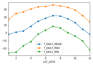
We can apply more customized aggregations, as with any groupby operation. Below we keep the mean of the mean, max of the max, and min of the min for the temperature measurements.

monthly_T_climatology = df.groupby(df.index.month).aggregate({'T_DAILY_MEAN': 'mean',
                                                              'T_DAILY_MAX': 'max',
                                                              'T_DAILY_MIN': 'min'})
monthly_T_climatology.head()

	T_DAILY_MEAN	T_DAILY_MAX	T_DAILY_MIN
LST_DATE
1	-2.100000	16.9	-26.0
2	0.712941	24.9	-24.7
3	2.455914	26.8	-16.5
4	8.302222	30.6	-11.3
5	14.850538	33.4	-1.6

monthly_T_climatology.plot(marker='o')

<matplotlib.axes._subplots.AxesSubplot at 0x10f0577b8>

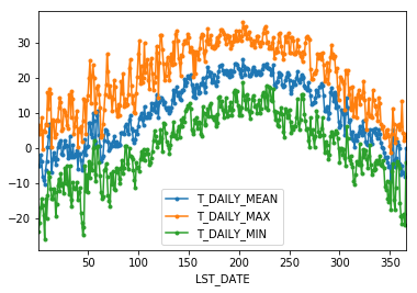
If we want to do it on a finer scale, we can group by day of year.

daily_T_climatology = df.groupby(df.index.dayofyear).aggregate({'T_DAILY_MEAN': 'mean',
                                                            'T_DAILY_MAX': 'max',
                                                            'T_DAILY_MIN': 'min'})
daily_T_climatology.plot(marker='.')

<matplotlib.axes._subplots.AxesSubplot at 0x1129e5c88>

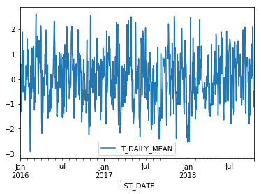
Calculating anomalies#

A common mode of analysis in climate science is to remove the climatology from a signal to focus only on the “anomaly” values. This can be accomplished with transformation.

def standardize(x):
    return (x - x.mean())/x.std()

anomaly = df.groupby(df.index.month).transform(standardize)
anomaly.plot(y='T_DAILY_MEAN')

/Users/rpa/miniconda3/envs/geo_scipy/lib/python3.6/site-packages/pandas/core/ops.py:692: RuntimeWarning: invalid value encountered in double_scalars
  lambda x: op(x, rvalues))

<matplotlib.axes._subplots.AxesSubplot at 0x10ef63828>

Resampling#

Another common operation is to change the resolution of a dataset by resampling in time. Pandas exposes this through the resample function. The resample periods are specified using pandas offset index syntax.

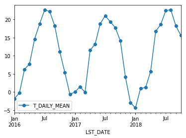
Below we resample the dataset by taking the mean over each month.

df.resample('M').mean().plot(y='T_DAILY_MEAN', marker='o')

<matplotlib.axes._subplots.AxesSubplot at 0x1126a5278>

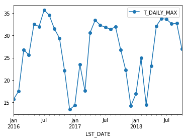
Just like with groupby, we can apply any aggregation function to our resample operation.

df.resample('M').max().plot(y='T_DAILY_MAX', marker='o')

<matplotlib.axes._subplots.AxesSubplot at 0x10efc6160>

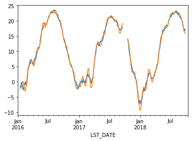
Rolling Operations#

The final category of operations applies to “rolling windows”. (See rolling documentation.) We specify a function to apply over a moving window along the index. We specify the size of the window and, optionally, the weights. We also use the keyword centered to tell pandas whether to center the operation around the midpoint of the window.

df.rolling(30, center=True).T_DAILY_MEAN.mean().plot()
df.rolling(30, center=True, win_type='triang').T_DAILY_MEAN.mean().plot()

<matplotlib.axes._subplots.AxesSubplot at 0x112cd4b38>

Earth and Environmental Data Science

Pandas: Groupby

Contents

Pandas: Groupby#

An Example#

What Happened?#

The `groupby` method#

The `GroubBy` object#

Iterating and selecting groups#

Aggregation#

Transformation#

Time Grouping#

Calculating anomalies#

Resampling#

Rolling Operations#

Earth and Environmental Data Science

Pandas: Groupby

Contents

Pandas: Groupby#

An Example#

What Happened?#

The groupby method#

The GroubBy object#

Iterating and selecting groups#

Aggregation#

Transformation#

Time Grouping#

Calculating anomalies#

Resampling#

Rolling Operations#

The `groupby` method#

The `GroubBy` object#