Computing with Dask
Contents
Computing with Dask#
Dask Arrays#
A dask array looks and feels a lot like a numpy array. However, a dask array doesn’t directly hold any data. Instead, it symbolically represents the computations needed to generate the data. Nothing is actually computed until the actual numerical values are needed. This mode of operation is called “lazy”; it allows one to build up complex, large calculations symbolically before turning them over the scheduler for execution.
If we want to create a numpy array of all ones, we do it like this:
import numpy as np
shape = (1000, 4000)
ones_np = np.ones(shape)
ones_np
array([[1., 1., 1., ..., 1., 1., 1.],
       [1., 1., 1., ..., 1., 1., 1.],
       [1., 1., 1., ..., 1., 1., 1.],
       ...,
       [1., 1., 1., ..., 1., 1., 1.],
       [1., 1., 1., ..., 1., 1., 1.],
       [1., 1., 1., ..., 1., 1., 1.]])
This array contains exactly 32 MB of data:
ones_np.nbytes / 1e6
32.0
Now let’s create the same array using dask’s array interface.
import dask.array as da
ones = da.ones(shape)
ones
|
The dask array representation reveals the concept of “chunks”. “Chunks” describes how the array is split into sub-arrays. We did not specify any chunks, so Dask just used one single chunk for the array. This is not much different from a numpy array at this point.
Specifying Chunks#
However, we could have split up the array into many chunks.
 source: Dask Array Documentation
There are several ways to specify chunks. In this lecture, we will use a block shape.
chunk_shape = (1000, 1000)
ones = da.ones(shape, chunks=chunk_shape)
ones
|
Notice that we just see a symbolic represetnation of the array, including its shape, dtype, and chunksize.
No data has been generated yet.
When we call .compute() on a dask array, the computation is trigger and the dask array becomes a numpy array.
ones.compute()
array([[1., 1., 1., ..., 1., 1., 1.],
       [1., 1., 1., ..., 1., 1., 1.],
       [1., 1., 1., ..., 1., 1., 1.],
       ...,
       [1., 1., 1., ..., 1., 1., 1.],
       [1., 1., 1., ..., 1., 1., 1.],
       [1., 1., 1., ..., 1., 1., 1.]])
In order to understand what happened when we called .compute(), we can visualize the dask graph, the symbolic operations that make up the array
ones.visualize()
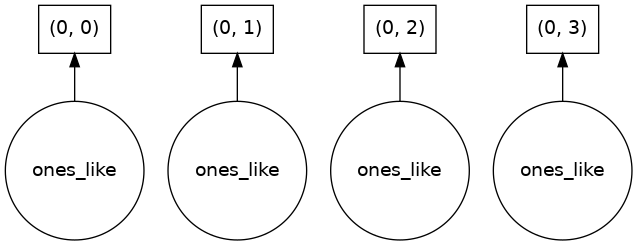
Our array has four chunks. To generate it, dask calls np.ones four times and then concatenates this together into one array.
Rather than immediately loading a dask array (which puts all the data into RAM), it is more common to want to reduce the data somehow. For example
sum_of_ones = ones.sum()
sum_of_ones.visualize()
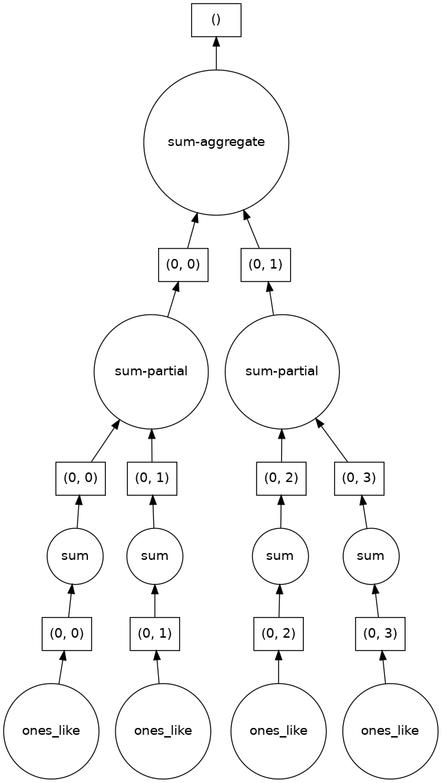
Here we see dask’s strategy for finding the sum. This simple example illustrates the beauty of dask: it automatically designs an algorithm appropriate for custom operations with big data.
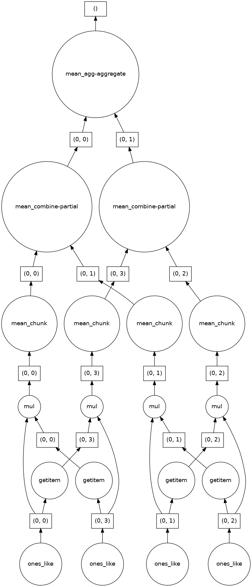
If we make our operation more complex, the graph gets more complex.
fancy_calculation = (ones * ones[::-1, ::-1]).mean()
fancy_calculation.visualize()
A Bigger Calculation#
The examples above were toy examples; the data (32 MB) is nowhere nearly big enough to warrant the use of dask.
We can make it a lot bigger!
bigshape = (200000, 4000)
big_ones = da.ones(bigshape, chunks=chunk_shape)
big_ones
|
big_ones.nbytes / 1e6
6400.0
This dataset is 3.2 GB, rather MB! This is probably close to or greater than the amount of available RAM than you have in your computer. Nevertheless, dask has no problem working on it.
Do not try to .visualize() this array!
When doing a big calculation, dask also has some tools to help us understand what is happening under the hood
from dask.diagnostics import ProgressBar

big_calc = (big_ones * big_ones[::-1, ::-1]).mean()

with ProgressBar():
    result = big_calc.compute()
result
[########################################] | 100% Completed | 2.4s
1.0
Reduction#
All the usual numpy methods work on dask arrays. You can also apply numpy function directly to a dask array, and it will stay lazy.
big_ones_reduce = (np.cos(big_ones)**2).mean(axis=0)
big_ones_reduce
|
Plotting also triggers computation, since we need the actual values
from matplotlib import pyplot as plt
%matplotlib inline
plt.rcParams['figure.figsize'] = (12,8)
plt.plot(big_ones_reduce)
[<matplotlib.lines.Line2D at 0x7f18689fbb80>]
Distributed Clusters#
Once we are ready to make a bigger calculation with dask, we can use a Dask Distributed cluster.
Warning
A common mistake is to move to distributed mode too soon. For smaller data, distributed will actually be much slower than the default multi-threaded scheduler or not using Dask at all. You should only use distributed when your data is much larger than what your computer can handle in memory.
Local Cluster#
A local cluster uses all the CPU cores of the machine it is running on. For our cloud-based Jupyterlab environments, that is just 2 cores–not very much. However, it’s good to know about.
from dask.distributed import Client, LocalCluster
cluster = LocalCluster()
client = Client(cluster)
client
Client
Client-0d54068d-5381-11ec-8481-f2f93f425864
| Connection method: Cluster object | Cluster type: distributed.LocalCluster |
| Dashboard: /user/rabernat/proxy/8787/status |
Cluster Info
LocalCluster
5a3ea957
| Dashboard: /user/rabernat/proxy/8787/status | Workers: 2 |
| Total threads: 2 | Total memory: 8.00 GiB |
| Status: running | Using processes: True |
Scheduler Info
Scheduler
Scheduler-1286f3af-8fb6-42d9-b7d0-61d90390e02f
| Comm: tcp://127.0.0.1:36005 | Workers: 2 |
| Dashboard: /user/rabernat/proxy/8787/status | Total threads: 2 |
| Started: Just now | Total memory: 8.00 GiB |
Workers
Worker: 0
| Comm: tcp://10.8.2.9:33951 | Total threads: 1 |
| Dashboard: /user/rabernat/proxy/38391/status | Memory: 4.00 GiB |
| Nanny: tcp://127.0.0.1:46605 | |
| Local directory: /home/jovyan/earth-env-data-science-book/src/lectures/dask/dask-worker-space/worker-cl1bqnsp | |
Worker: 1
| Comm: tcp://10.8.2.9:38345 | Total threads: 1 |
| Dashboard: /user/rabernat/proxy/33795/status | Memory: 4.00 GiB |
| Nanny: tcp://127.0.0.1:44415 | |
| Local directory: /home/jovyan/earth-env-data-science-book/src/lectures/dask/dask-worker-space/worker-iv640uvq | |
Note that the “Dashboard” link will open a new page where you can monitor a computation’s progress.
big_calc.compute()
1.0
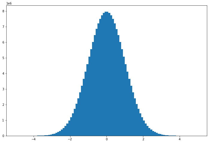
Here is another bigger calculation.
random_values = da.random.normal(size=(2e8,), chunks=(1e6,))
hist, bins = da.histogram(random_values, bins=100, range=[-5, 5])
hist
|
# actually trigger the computation
hist_c = hist.compute()
# plot results
x = 0.5 * (bins[1:] + bins[:-1])
width = np.diff(bins)
plt.bar(x, hist_c, width);
Dask Gateway - A Cluster in the Cloud#
Pangeo Cloud makes it possible to launch a much larger cluster using many virtual machines in the cloud. This is beyond the scope of our class, but you can read more about it in the Pangeo Cloud docs
Dask + XArray#
Xarray can automatically wrap its data in dask arrays. This capability turns xarray into an extremely powerful tool for Big Data earth science
To see this in action, we will open a dataset from the Pangeo Cloud Data Catalog - the Copernicus Sea Surface Height dataset.
from intake import open_catalog
cat = open_catalog("https://raw.githubusercontent.com/pangeo-data/pangeo-datastore/master/intake-catalogs/ocean.yaml")
ds  = cat["sea_surface_height"].to_dask()
ds
<xarray.Dataset>
Dimensions:    (time: 8901, latitude: 720, longitude: 1440, nv: 2)
Coordinates:
    crs        int32 ...
    lat_bnds   (time, latitude, nv) float32 dask.array<chunksize=(5, 720, 2), meta=np.ndarray>
  * latitude   (latitude) float32 -89.88 -89.62 -89.38 ... 89.38 89.62 89.88
    lon_bnds   (longitude, nv) float32 dask.array<chunksize=(1440, 2), meta=np.ndarray>
  * longitude  (longitude) float32 0.125 0.375 0.625 0.875 ... 359.4 359.6 359.9
  * nv         (nv) int32 0 1
  * time       (time) datetime64[ns] 1993-01-01 1993-01-02 ... 2017-05-15
Data variables:
    adt        (time, latitude, longitude) float64 dask.array<chunksize=(5, 720, 1440), meta=np.ndarray>
    err        (time, latitude, longitude) float64 dask.array<chunksize=(5, 720, 1440), meta=np.ndarray>
    sla        (time, latitude, longitude) float64 dask.array<chunksize=(5, 720, 1440), meta=np.ndarray>
    ugos       (time, latitude, longitude) float64 dask.array<chunksize=(5, 720, 1440), meta=np.ndarray>
    ugosa      (time, latitude, longitude) float64 dask.array<chunksize=(5, 720, 1440), meta=np.ndarray>
    vgos       (time, latitude, longitude) float64 dask.array<chunksize=(5, 720, 1440), meta=np.ndarray>
    vgosa      (time, latitude, longitude) float64 dask.array<chunksize=(5, 720, 1440), meta=np.ndarray>
Attributes: (12/43)
    Conventions:                     CF-1.6
    Metadata_Conventions:            Unidata Dataset Discovery v1.0
    cdm_data_type:                   Grid
    comment:                         Sea Surface Height measured by Altimetry...
    contact:                         servicedesk.cmems@mercator-ocean.eu
    creator_email:                   servicedesk.cmems@mercator-ocean.eu
    ...                              ...
    summary:                         SSALTO/DUACS Delayed-Time Level-4 sea su...
    time_coverage_duration:          P1D
    time_coverage_end:               1993-01-01T12:00:00Z
    time_coverage_resolution:        P1D
    time_coverage_start:             1992-12-31T12:00:00Z
title: DT merged all satellites Global Ocean Gr...- time: 8901
- latitude: 720
- longitude: 1440
- nv: 2
- crs()int32...
- comment :
- This is a container variable that describes the grid_mapping used by the data in this file. This variable does not contain any data; only information about the geographic coordinate system.
- grid_mapping_name :
- latitude_longitude
- inverse_flattening :
- 298.257
- semi_major_axis :
- 6378136.3
array(-2147483647, dtype=int32)
- lat_bnds(time, latitude, nv)float32dask.array<chunksize=(5, 720, 2), meta=np.ndarray>
- comment :
- latitude values at the north and south bounds of each pixel.
- units :
- degrees_north
Array Chunk Bytes 48.89 MiB 28.12 kiB Shape (8901, 720, 2) (5, 720, 2) Count 1782 Tasks 1781 Chunks Type float32 numpy.ndarray - latitude(latitude)float32-89.88 -89.62 ... 89.62 89.88
- axis :
- Y
- bounds :
- lat_bnds
- long_name :
- Latitude
- standard_name :
- latitude
- units :
- degrees_north
- valid_max :
- 89.875
- valid_min :
- -89.875
array([-89.875, -89.625, -89.375, ..., 89.375, 89.625, 89.875], dtype=float32) - lon_bnds(longitude, nv)float32dask.array<chunksize=(1440, 2), meta=np.ndarray>
- comment :
- longitude values at the west and east bounds of each pixel.
- units :
- degrees_east
Array Chunk Bytes 11.25 kiB 11.25 kiB Shape (1440, 2) (1440, 2) Count 2 Tasks 1 Chunks Type float32 numpy.ndarray - longitude(longitude)float320.125 0.375 0.625 ... 359.6 359.9
- axis :
- X
- bounds :
- lon_bnds
- long_name :
- Longitude
- standard_name :
- longitude
- units :
- degrees_east
- valid_max :
- 359.875
- valid_min :
- 0.125
array([1.25000e-01, 3.75000e-01, 6.25000e-01, ..., 3.59375e+02, 3.59625e+02, 3.59875e+02], dtype=float32) - nv(nv)int320 1
- comment :
- Vertex
- units :
- 1
array([0, 1], dtype=int32)
- time(time)datetime64[ns]1993-01-01 ... 2017-05-15
- axis :
- T
- long_name :
- Time
- standard_name :
- time
array(['1993-01-01T00:00:00.000000000', '1993-01-02T00:00:00.000000000',
       '1993-01-03T00:00:00.000000000', ..., '2017-05-13T00:00:00.000000000',
       '2017-05-14T00:00:00.000000000', '2017-05-15T00:00:00.000000000'],
      dtype='datetime64[ns]')
- adt(time, latitude, longitude)float64dask.array<chunksize=(5, 720, 1440), meta=np.ndarray>
- comment :
- The absolute dynamic topography is the sea surface height above geoid; the adt is obtained as follows: adt=sla+mdt where mdt is the mean dynamic topography; see the product user manual for details
- grid_mapping :
- crs
- long_name :
- Absolute dynamic topography
- standard_name :
- sea_surface_height_above_geoid
- units :
- m
Array Chunk Bytes 68.76 GiB 39.55 MiB Shape (8901, 720, 1440) (5, 720, 1440) Count 1782 Tasks 1781 Chunks Type float64 numpy.ndarray - err(time, latitude, longitude)float64dask.array<chunksize=(5, 720, 1440), meta=np.ndarray>
- comment :
- The formal mapping error represents a purely theoretical mapping error. It mainly traduces errors induced by the constellation sampling capability and consistency with the spatial/temporal scales considered, as described in Le Traon et al (1998) or Ducet et al (2000)
- grid_mapping :
- crs
- long_name :
- Formal mapping error
- units :
- m
Array Chunk Bytes 68.76 GiB 39.55 MiB Shape (8901, 720, 1440) (5, 720, 1440) Count 1782 Tasks 1781 Chunks Type float64 numpy.ndarray - sla(time, latitude, longitude)float64dask.array<chunksize=(5, 720, 1440), meta=np.ndarray>
- comment :
- The sea level anomaly is the sea surface height above mean sea surface; it is referenced to the [1993, 2012] period; see the product user manual for details
- grid_mapping :
- crs
- long_name :
- Sea level anomaly
- standard_name :
- sea_surface_height_above_sea_level
- units :
- m
Array Chunk Bytes 68.76 GiB 39.55 MiB Shape (8901, 720, 1440) (5, 720, 1440) Count 1782 Tasks 1781 Chunks Type float64 numpy.ndarray - ugos(time, latitude, longitude)float64dask.array<chunksize=(5, 720, 1440), meta=np.ndarray>
- grid_mapping :
- crs
- long_name :
- Absolute geostrophic velocity: zonal component
- standard_name :
- surface_geostrophic_eastward_sea_water_velocity
- units :
- m/s
Array Chunk Bytes 68.76 GiB 39.55 MiB Shape (8901, 720, 1440) (5, 720, 1440) Count 1782 Tasks 1781 Chunks Type float64 numpy.ndarray - ugosa(time, latitude, longitude)float64dask.array<chunksize=(5, 720, 1440), meta=np.ndarray>
- comment :
- The geostrophic velocity anomalies are referenced to the [1993, 2012] period
- grid_mapping :
- crs
- long_name :
- Geostrophic velocity anomalies: zonal component
- standard_name :
- surface_geostrophic_eastward_sea_water_velocity_assuming_sea_level_for_geoid
- units :
- m/s
Array Chunk Bytes 68.76 GiB 39.55 MiB Shape (8901, 720, 1440) (5, 720, 1440) Count 1782 Tasks 1781 Chunks Type float64 numpy.ndarray - vgos(time, latitude, longitude)float64dask.array<chunksize=(5, 720, 1440), meta=np.ndarray>
- grid_mapping :
- crs
- long_name :
- Absolute geostrophic velocity: meridian component
- standard_name :
- surface_geostrophic_northward_sea_water_velocity
- units :
- m/s
Array Chunk Bytes 68.76 GiB 39.55 MiB Shape (8901, 720, 1440) (5, 720, 1440) Count 1782 Tasks 1781 Chunks Type float64 numpy.ndarray - vgosa(time, latitude, longitude)float64dask.array<chunksize=(5, 720, 1440), meta=np.ndarray>
- comment :
- The geostrophic velocity anomalies are referenced to the [1993, 2012] period
- grid_mapping :
- crs
- long_name :
- Geostrophic velocity anomalies: meridian component
- standard_name :
- surface_geostrophic_northward_sea_water_velocity_assuming_sea_level_for_geoid
- units :
- m/s
Array Chunk Bytes 68.76 GiB 39.55 MiB Shape (8901, 720, 1440) (5, 720, 1440) Count 1782 Tasks 1781 Chunks Type float64 numpy.ndarray
- Conventions :
- CF-1.6
- Metadata_Conventions :
- Unidata Dataset Discovery v1.0
- cdm_data_type :
- Grid
- comment :
- Sea Surface Height measured by Altimetry and derived variables
- contact :
- servicedesk.cmems@mercator-ocean.eu
- creator_email :
- servicedesk.cmems@mercator-ocean.eu
- creator_name :
- CMEMS - Sea Level Thematic Assembly Center
- creator_url :
- http://marine.copernicus.eu
- date_created :
- 2014-02-26T16:09:13Z
- date_issued :
- 2014-01-06T00:00:00Z
- date_modified :
- 2015-11-10T19:42:51Z
- geospatial_lat_max :
- 89.875
- geospatial_lat_min :
- -89.875
- geospatial_lat_resolution :
- 0.25
- geospatial_lat_units :
- degrees_north
- geospatial_lon_max :
- 359.875
- geospatial_lon_min :
- 0.125
- geospatial_lon_resolution :
- 0.25
- geospatial_lon_units :
- degrees_east
- geospatial_vertical_max :
- 0.0
- geospatial_vertical_min :
- 0.0
- geospatial_vertical_positive :
- down
- geospatial_vertical_resolution :
- point
- geospatial_vertical_units :
- m
- history :
- 2014-02-26T16:09:13Z: created by DUACS DT - 2015-11-10T19:42:51Z: Change of some attributes - 2017-01-06 12:12:12Z: New format for CMEMSv3
- institution :
- CLS, CNES
- keywords :
- Oceans > Ocean Topography > Sea Surface Height
- keywords_vocabulary :
- NetCDF COARDS Climate and Forecast Standard Names
- license :
- http://marine.copernicus.eu/web/27-service-commitments-and-licence.php
- platform :
- ERS-1, Topex/Poseidon
- processing_level :
- L4
- product_version :
- 5.0
- project :
- COPERNICUS MARINE ENVIRONMENT MONITORING SERVICE (CMEMS)
- references :
- http://marine.copernicus.eu
- source :
- Altimetry measurements
- ssalto_duacs_comment :
- The reference mission used for the altimeter inter-calibration processing is Topex/Poseidon between 1993-01-01 and 2002-04-23, Jason-1 between 2002-04-24 and 2008-10-18, OSTM/Jason-2 since 2008-10-19.
- standard_name_vocabulary :
- NetCDF Climate and Forecast (CF) Metadata Convention Standard Name Table v37
- summary :
- SSALTO/DUACS Delayed-Time Level-4 sea surface height and derived variables measured by multi-satellite altimetry observations over Global Ocean.
- time_coverage_duration :
- P1D
- time_coverage_end :
- 1993-01-01T12:00:00Z
- time_coverage_resolution :
- P1D
- time_coverage_start :
- 1992-12-31T12:00:00Z
- title :
- DT merged all satellites Global Ocean Gridded SSALTO/DUACS Sea Surface Height L4 product and derived variables
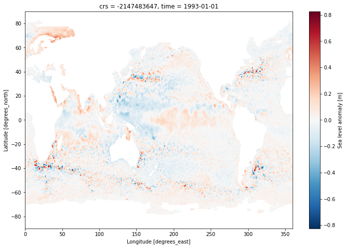
Note that the values are not displayed, since that would trigger computation.
ds.sla[0].plot()
<matplotlib.collections.QuadMesh at 0x7f17ae3e4f10>
# the computationally intensive step
sla_timeseries = ds.sla.mean(dim=('latitude', 'longitude')).load()
sla_timeseries.plot(label='full data')
sla_timeseries.rolling(time=365, center=True).mean().plot(label='rolling annual mean')
plt.ylabel('Sea Level Anomaly [m]')
plt.title('Global Mean Sea Level')
plt.legend()
plt.grid()