Working with output from many different CMIP6 climate models

Climate modeling has been a cornerstone of understanding our climate and the consequences of continued emissions of greenhouse gases for decades. Much of the recent efforts in the community have been focus on model intercomparison projects (MIPs), which invite submissions of many different modeling groups around the world to run their models (which are all set up slightly different) under centralized forcing scenarios. These results can then be analyzed and the spread between different models can give an idea about the certainty of these predictions. The recent Coupled Model Intercomparison Project Phase 6 (CMIP6) represents an international effort to represent the state-of-the-art knowledge about how the climate system might evolve in the future and informs much of the [Intergovernmental Panel on Climate Change Report](Intergovernmental Panel on Climate Change Report.

In this lecture we will learn how to quickly search and analyze CMIP6 data with Pangeo tools in the cloud, a process that using the ‘download and analyze’ workflow often becomes prohibitively slow and inefficient due to the sheer scale of the data.

The basis for this workflow are the analysis-ready-cloud-optimized repositories of CMIP6 data, which are currently maintained by the pangeo community and publicly available on both Google Cloud Storage and Amazon S3 as a collection of zarr stores.

The cloud native approach enables scientific results to be fully reproducible, encouraging to build onto and collaborate on scientific results.

from xmip.preprocessing import combined_preprocessing
from xmip.utils import google_cmip_col
from xmip.postprocessing import match_metrics
import matplotlib.pyplot as plt

The first thing we have to do is to get an overview of all the data available. In this case we are using intake-esm to load a collection of zarr stores on Google Cloud Storage, but there are other options to access the data too.

Lets create a collection object and look at it

col = google_cmip_col()
col

pangeo-cmip6 catalog with 7674 dataset(s) from 514818 asset(s):

	unique
activity_id	18
institution_id	36
source_id	88
experiment_id	170
member_id	657
table_id	37
variable_id	700
grid_label	10
zstore	514818
dcpp_init_year	60
version	736
derived_variable_id	0

This object describes all the available data (over 500k single zarr stores!). The rows describe different ‘facets’ that can be used to search and query subsets of the data. For detailed info on each of the facets please refer to this document.

So obviously we never want to work with all the data. Lets check out how to get a subset.

First we need to understand a bit better what all these facets mean and how to see which ones are in the full collection. Lets start with the experiment_id: This is the prescribed forcing for a particular MIP that is exactly the same across all different models. We can look at the values of the collection as a pandas dataframe to convieniently list all values.

col.df['experiment_id'].unique()

array(['highresSST-present', 'piControl', 'control-1950', 'hist-1950',
       'historical', 'amip', 'abrupt-4xCO2', 'abrupt-2xCO2',
       'abrupt-0p5xCO2', '1pctCO2', 'ssp585', 'esm-piControl', 'esm-hist',
       'hist-piAer', 'histSST-1950HC', 'ssp245', 'hist-1950HC', 'histSST',
       'piClim-2xVOC', 'piClim-2xNOx', 'piClim-2xdust', 'piClim-2xss',
       'piClim-histall', 'hist-piNTCF', 'histSST-piNTCF',
       'aqua-control-lwoff', 'piClim-lu', 'histSST-piO3', 'piClim-CH4',
       'piClim-NTCF', 'piClim-NOx', 'piClim-O3', 'piClim-HC',
       'faf-heat-NA0pct', 'ssp370SST-lowCH4', 'piClim-VOC',
       'ssp370-lowNTCF', 'piClim-control', 'piClim-aer', 'hist-aer',
       'faf-heat', 'faf-heat-NA50pct', 'ssp370SST-lowNTCF',
       'ssp370SST-ssp126Lu', 'ssp370SST', 'ssp370pdSST', 'histSST-piAer',
       'piClim-ghg', 'piClim-anthro', 'faf-all', 'hist-nat', 'hist-GHG',
       'ssp119', 'piClim-histnat', 'piClim-4xCO2', 'ssp370',
       'piClim-histghg', 'highresSST-future', 'esm-ssp585-ssp126Lu',
       'ssp126-ssp370Lu', 'ssp370-ssp126Lu', 'land-noLu', 'histSST-piCH4',
       'ssp126', 'esm-pi-CO2pulse', 'amip-hist', 'piClim-histaer',
       'amip-4xCO2', 'faf-water', 'faf-passiveheat', '1pctCO2-rad',
       'faf-stress', '1pctCO2-bgc', 'aqua-control', 'amip-future4K',
       'amip-p4K', 'aqua-p4K', 'amip-lwoff', 'amip-m4K', 'aqua-4xCO2',
       'amip-p4K-lwoff', 'hist-noLu', '1pctCO2-cdr',
       'land-hist-altStartYear', 'land-hist', 'omip1', 'esm-pi-cdr-pulse',
       'esm-ssp585', 'abrupt-solp4p', 'piControl-spinup', 'hist-stratO3',
       'abrupt-solm4p', 'midHolocene', 'lig127k', 'aqua-p4K-lwoff',
       'esm-piControl-spinup', 'ssp245-GHG', 'ssp245-nat',
       'dcppC-amv-neg', 'dcppC-amv-ExTrop-neg', 'dcppC-atl-control',
       'dcppC-amv-pos', 'dcppC-ipv-NexTrop-neg', 'dcppC-ipv-NexTrop-pos',
       'dcppC-atl-pacemaker', 'dcppC-amv-ExTrop-pos',
       'dcppC-amv-Trop-neg', 'dcppC-pac-control', 'dcppC-ipv-pos',
       'dcppC-pac-pacemaker', 'dcppC-ipv-neg', 'dcppC-amv-Trop-pos',
       'piClim-BC', 'piClim-2xfire', 'piClim-SO2', 'piClim-OC',
       'piClim-N2O', 'piClim-2xDMS', 'ssp460', 'ssp434', 'ssp534-over',
       'deforest-globe', 'historical-cmip5', 'hist-bgc',
       'piControl-cmip5', 'rcp26-cmip5', 'rcp45-cmip5', 'rcp85-cmip5',
       'pdSST-piArcSIC', 'pdSST-piAntSIC', 'piSST-piSIC', 'piSST-pdSIC',
       'ssp245-stratO3', 'hist-sol', 'hist-CO2', 'hist-volc',
       'hist-totalO3', 'hist-nat-cmip5', 'hist-aer-cmip5',
       'hist-GHG-cmip5', 'pdSST-futAntSIC', 'futSST-pdSIC', 'pdSST-pdSIC',
       'ssp245-aer', 'pdSST-futArcSIC', 'dcppA-hindcast', 'dcppA-assim',
       'dcppC-hindcast-noPinatubo', 'dcppC-hindcast-noElChichon',
       'dcppC-hindcast-noAgung', 'ssp245-cov-modgreen',
       'ssp245-cov-fossil', 'ssp245-cov-strgreen', 'ssp245-covid', 'lgm',
       'ssp585-bgc', '1pctCO2to4x-withism', '1pctCO2-4xext',
       'hist-resIPO', 'past1000', 'pa-futArcSIC', 'pa-pdSIC',
       'historical-ext', 'pdSST-futArcSICSIT', 'pdSST-futOkhotskSIC',
       'pdSST-futBKSeasSIC', 'pa-piArcSIC', 'pa-piAntSIC', 'pa-futAntSIC',
       'pdSST-pdSICSIT'], dtype=object)

The experiments you are probably most interested in are the following:

• piControl: In most cases this is the ‘spin up’ phase of the model, where it is run with a constant forcing (representing pre-industrial greenhouse gas concentrations)

• historical: This experiment is run with the observed forcing in the past.

• ssp***: A set of “Shared Socioeconomic Pathways” which represent different combined scenarios of future greenhouse gas emissions and other socio-economic indicators (Explainer). These are a fairly complex topic, but to simplify this for our purposes here we can treat ssp585 as the ‘worst-case’ and ssp245 as ‘middle-of-the-road’.

You can explore the available models (source_id) in the same way as above:

col.df['source_id'].unique()

array(['CMCC-CM2-HR4', 'EC-Earth3P-HR', 'HadGEM3-GC31-MM',
       'HadGEM3-GC31-HM', 'HadGEM3-GC31-LM', 'EC-Earth3P', 'ECMWF-IFS-HR',
       'ECMWF-IFS-LR', 'HadGEM3-GC31-LL', 'CMCC-CM2-VHR4', 'GFDL-CM4',
       'GFDL-AM4', 'IPSL-CM6A-LR', 'E3SM-1-0', 'CNRM-CM6-1', 'GFDL-ESM4',
       'GFDL-ESM2M', 'GFDL-CM4C192', 'GFDL-OM4p5B', 'GISS-E2-1-G',
       'GISS-E2-1-H', 'CNRM-ESM2-1', 'BCC-CSM2-MR', 'BCC-ESM1', 'MIROC6',
       'AWI-CM-1-1-MR', 'EC-Earth3-LR', 'IPSL-CM6A-ATM-HR', 'CESM2',
       'CESM2-WACCM', 'CNRM-CM6-1-HR', 'MRI-ESM2-0', 'SAM0-UNICON',
       'GISS-E2-1-G-CC', 'UKESM1-0-LL', 'EC-Earth3', 'EC-Earth3-Veg',
       'FGOALS-f3-L', 'CanESM5', 'CanESM5-CanOE', 'INM-CM4-8',
       'INM-CM5-0', 'NESM3', 'MPI-ESM-1-2-HAM', 'CAMS-CSM1-0',
       'MPI-ESM1-2-LR', 'MPI-ESM1-2-HR', 'MRI-AGCM3-2-H', 'MRI-AGCM3-2-S',
       'MCM-UA-1-0', 'INM-CM5-H', 'KACE-1-0-G', 'NorESM2-LM',
       'FGOALS-f3-H', 'FGOALS-g3', 'MIROC-ES2L', 'FIO-ESM-2-0', 'NorCPM1',
       'NorESM1-F', 'MPI-ESM1-2-XR', 'CESM1-1-CAM5-CMIP5', 'E3SM-1-1',
       'KIOST-ESM', 'ACCESS-CM2', 'NorESM2-MM', 'ACCESS-ESM1-5',
       'IITM-ESM', 'GISS-E2-2-G', 'CESM2-FV2', 'GISS-E2-2-H',
       'CESM2-WACCM-FV2', 'CIESM', 'E3SM-1-1-ECA', 'TaiESM1',
       'AWI-ESM-1-1-LR', 'EC-Earth3-Veg-LR', 'CMCC-ESM2', 'CMCC-CM2-SR5',
       'EC-Earth3-AerChem', 'IPSL-CM6A-LR-INCA', 'IPSL-CM5A2-INCA',
       'BCC-CSM2-HR', 'EC-Earth3P-VHR', 'CESM1-WACCM-SC', 'CAS-ESM2-0',
       'EC-Earth3-CC', 'MIROC-ES2H', 'ICON-ESM-LR'], dtype=object)

Now you want to decide what variable (variable_id) you want to look at and in conjunction what time frequency of output (table_id) is available. This handy spreadsheet can help you find the value for variable_id and the available time frequencies (table_id).

Lets look at an example for monthly ('table_id'='Omon') sea surface temperature ('variable_id'='tos') for the historical experiment:

cat = col.search(
    variable_id='tos', # ocean surface temperature
    table_id='Omon',
    experiment_id='historical',
    source_id=['GFDL-ESM4'],
)
cat

pangeo-cmip6 catalog with 2 dataset(s) from 6 asset(s):

	unique
activity_id	1
institution_id	1
source_id	1
experiment_id	1
member_id	3
table_id	1
variable_id	1
grid_label	2
zstore	6
dcpp_init_year	0
version	2
derived_variable_id	0

The last facet we need to discuss is member_id and grid_label: You can see here that we have 3 member_id values for the given query.

cat.df['member_id'].unique()

array(['r3i1p1f1', 'r2i1p1f1', 'r1i1p1f1'], dtype=object)

This indicates that for this particular model/experiment 3 ensemble members where run with varing realizations/initial_condiditions/physics/forcing or a combination thereof. The naming is explained in thisdocument:

Example of a variant_label: if realization_index=2, initialization_index=1, physics_index=3, and forcing_index=233, then variant_label = “r2i1p3f233”.

There can be many more members for some particular models, which provides an opportunity to investigate internal variability of the climate system as compared to forced signals.

Finally there are two values of grid_label

cat.df['grid_label'].unique()

array(['gr', 'gn'], dtype=object)

The value gn always stands for the native model grid (which can be quite complex but preserves the most detail) and gr indicates data that has been regridded on regular lon/lat intervals.

Now that you know how to query and subset the collection, it is time to actually load in some model data as xarray datasets!

# create a smaller catalog from the full collection using faceted search
cat = col.search(
    variable_id='tos', # Ocean surface temperature
    experiment_id='historical', # only runs for the historical forcing period
    table_id='Omon', # monthly oceanic data
    grid_label='gn', #native model grid only
    source_id=['IPSL-CM6A-LR', 'MRI-ESM2-0', 'GFDL-ESM4'], # only choosing a few models here, there are many more!
    member_id=['r1i1p1f1', 'r2i1p1f1', 'r3i1p1f1'], #lets restrict us here to only a few members, you can modify this later to experiment.
)

# read all datasets into a dictionary but apply the xmip preprocessing before
ddict = cat.to_dataset_dict(
    preprocess=combined_preprocessing,
    xarray_open_kwargs={'use_cftime':True},
)

--> The keys in the returned dictionary of datasets are constructed as follows:
	'activity_id.institution_id.source_id.experiment_id.table_id.grid_label'

100.00% [3/3 00:03<00:00]

/srv/conda/envs/notebook/lib/python3.9/site-packages/xmip/preprocessing.py:106: UserWarning: Renaming failed with 'area'
  warnings.warn(f"Renaming failed with {e}")
/srv/conda/envs/notebook/lib/python3.9/site-packages/xmip/preprocessing.py:106: UserWarning: Renaming failed with 'time_bounds'
  warnings.warn(f"Renaming failed with {e}")
/srv/conda/envs/notebook/lib/python3.9/site-packages/xmip/preprocessing.py:106: UserWarning: Renaming failed with 'tos'
  warnings.warn(f"Renaming failed with {e}")
/srv/conda/envs/notebook/lib/python3.9/site-packages/xmip/preprocessing.py:106: UserWarning: Renaming failed with 'tos'
  warnings.warn(f"Renaming failed with {e}")
/srv/conda/envs/notebook/lib/python3.9/site-packages/xmip/preprocessing.py:106: UserWarning: Renaming failed with the new name 'lon_bounds' conflicts
  warnings.warn(f"Renaming failed with {e}")
/srv/conda/envs/notebook/lib/python3.9/site-packages/xmip/preprocessing.py:106: UserWarning: Renaming failed with the new name 'lat_bounds' conflicts
  warnings.warn(f"Renaming failed with {e}")
/srv/conda/envs/notebook/lib/python3.9/site-packages/xmip/preprocessing.py:83: UserWarning: rename 'bnds' to 'bnds' does not create an index anymore. Try using swap_dims instead or use set_index after rename to create an indexed coordinate.
  return obj.rename({kk: vv for kk, vv in rdict.items() if kk in obj.dims})
/srv/conda/envs/notebook/lib/python3.9/site-packages/xmip/preprocessing.py:106: UserWarning: Renaming failed with 'lat'
  warnings.warn(f"Renaming failed with {e}")
/srv/conda/envs/notebook/lib/python3.9/site-packages/xmip/preprocessing.py:106: UserWarning: Renaming failed with 'lon'
  warnings.warn(f"Renaming failed with {e}")
/srv/conda/envs/notebook/lib/python3.9/site-packages/xmip/preprocessing.py:106: UserWarning: Renaming failed with 'tos'
  warnings.warn(f"Renaming failed with {e}")
/srv/conda/envs/notebook/lib/python3.9/site-packages/xmip/preprocessing.py:106: UserWarning: Renaming failed with 'area'
  warnings.warn(f"Renaming failed with {e}")
/srv/conda/envs/notebook/lib/python3.9/site-packages/xmip/preprocessing.py:106: UserWarning: Renaming failed with 'time_bounds'
  warnings.warn(f"Renaming failed with {e}")
/srv/conda/envs/notebook/lib/python3.9/site-packages/xmip/preprocessing.py:106: UserWarning: Renaming failed with 'tos'
  warnings.warn(f"Renaming failed with {e}")
/srv/conda/envs/notebook/lib/python3.9/site-packages/xmip/preprocessing.py:106: UserWarning: Renaming failed with 'tos'
  warnings.warn(f"Renaming failed with {e}")
/srv/conda/envs/notebook/lib/python3.9/site-packages/xmip/preprocessing.py:106: UserWarning: Renaming failed with the new name 'lon_bounds' conflicts
  warnings.warn(f"Renaming failed with {e}")
/srv/conda/envs/notebook/lib/python3.9/site-packages/xmip/preprocessing.py:106: UserWarning: Renaming failed with the new name 'lat_bounds' conflicts
  warnings.warn(f"Renaming failed with {e}")
/srv/conda/envs/notebook/lib/python3.9/site-packages/xmip/preprocessing.py:83: UserWarning: rename 'bnds' to 'bnds' does not create an index anymore. Try using swap_dims instead or use set_index after rename to create an indexed coordinate.
  return obj.rename({kk: vv for kk, vv in rdict.items() if kk in obj.dims})
/srv/conda/envs/notebook/lib/python3.9/site-packages/xmip/preprocessing.py:106: UserWarning: Renaming failed with 'lat'
  warnings.warn(f"Renaming failed with {e}")
/srv/conda/envs/notebook/lib/python3.9/site-packages/xmip/preprocessing.py:106: UserWarning: Renaming failed with 'lon'
  warnings.warn(f"Renaming failed with {e}")
/srv/conda/envs/notebook/lib/python3.9/site-packages/xmip/preprocessing.py:106: UserWarning: Renaming failed with 'tos'
  warnings.warn(f"Renaming failed with {e}")
/srv/conda/envs/notebook/lib/python3.9/site-packages/xmip/preprocessing.py:106: UserWarning: Renaming failed with 'area'
  warnings.warn(f"Renaming failed with {e}")
/srv/conda/envs/notebook/lib/python3.9/site-packages/xmip/preprocessing.py:106: UserWarning: Renaming failed with 'time_bounds'
  warnings.warn(f"Renaming failed with {e}")
/srv/conda/envs/notebook/lib/python3.9/site-packages/xmip/preprocessing.py:106: UserWarning: Renaming failed with 'tos'
  warnings.warn(f"Renaming failed with {e}")
/srv/conda/envs/notebook/lib/python3.9/site-packages/xmip/preprocessing.py:106: UserWarning: Renaming failed with 'tos'
  warnings.warn(f"Renaming failed with {e}")
/srv/conda/envs/notebook/lib/python3.9/site-packages/xmip/preprocessing.py:106: UserWarning: Renaming failed with the new name 'lon_bounds' conflicts
  warnings.warn(f"Renaming failed with {e}")
/srv/conda/envs/notebook/lib/python3.9/site-packages/xmip/preprocessing.py:106: UserWarning: Renaming failed with the new name 'lat_bounds' conflicts
  warnings.warn(f"Renaming failed with {e}")
/srv/conda/envs/notebook/lib/python3.9/site-packages/xmip/preprocessing.py:83: UserWarning: rename 'bnds' to 'bnds' does not create an index anymore. Try using swap_dims instead or use set_index after rename to create an indexed coordinate.
  return obj.rename({kk: vv for kk, vv in rdict.items() if kk in obj.dims})
/srv/conda/envs/notebook/lib/python3.9/site-packages/xmip/preprocessing.py:106: UserWarning: Renaming failed with 'lat'
  warnings.warn(f"Renaming failed with {e}")
/srv/conda/envs/notebook/lib/python3.9/site-packages/xmip/preprocessing.py:106: UserWarning: Renaming failed with 'lon'
  warnings.warn(f"Renaming failed with {e}")
/srv/conda/envs/notebook/lib/python3.9/site-packages/xmip/preprocessing.py:106: UserWarning: Renaming failed with 'tos'
  warnings.warn(f"Renaming failed with {e}")

Here we did two things:

• We searched the full collection based on a combination of facets like the variable, the experiment and only a test set of models.

• We loaded the datasets into a dictionary of xarray datasets (note they are not loaded into memory, but instead these are lazyly loaded dask arrays – more on this in the following lectures).

list(ddict.keys())

['CMIP.IPSL.IPSL-CM6A-LR.historical.Omon.gn',
 'CMIP.MRI.MRI-ESM2-0.historical.Omon.gn',
 'CMIP.NOAA-GFDL.GFDL-ESM4.historical.Omon.gn']

You can see that we have three different models. Lets look at them in a bit more detail to understand the layout:

ddict['CMIP.IPSL.IPSL-CM6A-LR.historical.Omon.gn']

<xarray.Dataset>
Dimensions:         (y: 332, x: 362, member_id: 3, dcpp_init_year: 1,
                     time: 1980, vertex: 4, bnds: 2)
Coordinates: (12/13)
    area            (y, x) float32 dask.array<chunksize=(332, 362), meta=np.ndarray>
    lat_verticies   (y, x, vertex) float32 dask.array<chunksize=(332, 362, 4), meta=np.ndarray>
    lon_verticies   (y, x, vertex) float32 dask.array<chunksize=(332, 362, 4), meta=np.ndarray>
    lat             (y, x) float32 dask.array<chunksize=(332, 362), meta=np.ndarray>
    lon             (y, x) float32 dask.array<chunksize=(332, 362), meta=np.ndarray>
  * time            (time) object 1850-01-16 12:00:00 ... 2014-12-16 12:00:00
    ...              ...
  * y               (y) int64 0 1 2 3 4 5 6 7 ... 325 326 327 328 329 330 331
  * x               (x) int64 0 1 2 3 4 5 6 7 ... 355 356 357 358 359 360 361
    lon_bounds      (bnds, y, x) float32 dask.array<chunksize=(1, 332, 362), meta=np.ndarray>
    lat_bounds      (bnds, y, x) float32 dask.array<chunksize=(1, 332, 362), meta=np.ndarray>
  * member_id       (member_id) object 'r1i1p1f1' 'r2i1p1f1' 'r3i1p1f1'
  * dcpp_init_year  (dcpp_init_year) float64 nan
Dimensions without coordinates: vertex, bnds
Data variables:
    tos             (member_id, dcpp_init_year, time, y, x) float32 dask.array<chunksize=(1, 1, 251, 332, 362), meta=np.ndarray>
Attributes: (12/52)
    CMIP6_CV_version:                 cv=6.2.3.5-2-g63b123e
    Conventions:                      CF-1.7 CMIP-6.2
    EXPID:                            historical
    NCO:                              "4.6.0"
    activity_id:                      CMIP
    branch_method:                    standard
    ...                               ...
    intake_esm_attrs:variable_id:     tos
    intake_esm_attrs:grid_label:      gn
    intake_esm_attrs:version:         20180803
    intake_esm_attrs:_data_format_:   zarr
    variant_info:                     Restart from another point in piControl...
    intake_esm_dataset_key:           CMIP.IPSL.IPSL-CM6A-LR.historical.Omon.gn

xarray.Dataset

• Dimensions:
  • y: 332
  • x: 362
  • member_id: 3
  • dcpp_init_year: 1
  • time: 1980
  • vertex: 4
  • bnds: 2
• Coordinates: (13)
  • area
    (y, x)
    float32
    dask.array<chunksize=(332, 362), meta=np.ndarray>

    standard_name :

    cell_area

    units :

    m²

    Array Chunk Bytes 469.47 kiB 469.47 kiB Shape (332, 362) (332, 362) Count 10 Graph Layers 1 Chunks Type float32 numpy.ndarray

  • lat_verticies
    (y, x, vertex)
    float32
    dask.array<chunksize=(332, 362, 4), meta=np.ndarray>

    Array Chunk Bytes 1.83 MiB 1.83 MiB Shape (332, 362, 4) (332, 362, 4) Count 12 Graph Layers 1 Chunks Type float32 numpy.ndarray

  • lon_verticies
    (y, x, vertex)
    float32
    dask.array<chunksize=(332, 362, 4), meta=np.ndarray>

    Array Chunk Bytes 1.83 MiB 1.83 MiB Shape (332, 362, 4) (332, 362, 4) Count 18 Graph Layers 1 Chunks Type float32 numpy.ndarray

  • lat
    (y, x)
    float32
    dask.array<chunksize=(332, 362), meta=np.ndarray>

    bounds :

    bounds_nav_lat

    long_name :

    Latitude

    standard_name :

    latitude

    units :

    degrees_north

    Array Chunk Bytes 469.47 kiB 469.47 kiB Shape (332, 362) (332, 362) Count 16 Graph Layers 1 Chunks Type float32 numpy.ndarray

  • lon
    (y, x)
    float32
    dask.array<chunksize=(332, 362), meta=np.ndarray>

    bounds :

    bounds_nav_lon

    long_name :

    Longitude

    standard_name :

    longitude

    units :

    degrees_east

    Array Chunk Bytes 469.47 kiB 469.47 kiB Shape (332, 362) (332, 362) Count 22 Graph Layers 1 Chunks Type float32 numpy.ndarray

  • time
    (time)
    object
    1850-01-16 12:00:00 ... 2014-12-...

    axis :

    T

    bounds :

    time_bounds

    long_name :

    Time axis

    standard_name :

    time

    time_origin :

    1850-01-01 00:00:00

    array([cftime.DatetimeGregorian(1850, 1, 16, 12, 0, 0, 0, has_year_zero=False),
           cftime.DatetimeGregorian(1850, 2, 15, 0, 0, 0, 0, has_year_zero=False),
           cftime.DatetimeGregorian(1850, 3, 16, 12, 0, 0, 0, has_year_zero=False),
           ...,
           cftime.DatetimeGregorian(2014, 10, 16, 12, 0, 0, 0, has_year_zero=False),
           cftime.DatetimeGregorian(2014, 11, 16, 0, 0, 0, 0, has_year_zero=False),
           cftime.DatetimeGregorian(2014, 12, 16, 12, 0, 0, 0, has_year_zero=False)],
          dtype=object)

  • time_bounds
    (time, bnds)
    object
    dask.array<chunksize=(1980, 2), meta=np.ndarray>

    Array Chunk Bytes 30.94 kiB 30.94 kiB Shape (1980, 2) (1980, 2) Count 10 Graph Layers 1 Chunks Type object numpy.ndarray

  • y
    (y)
    int64
    0 1 2 3 4 5 ... 327 328 329 330 331

    array([  0,   1,   2, ..., 329, 330, 331])

  • x
    (x)
    int64
    0 1 2 3 4 5 ... 357 358 359 360 361

    array([  0,   1,   2, ..., 359, 360, 361])

  • lon_bounds
    (bnds, y, x)
    float32
    dask.array<chunksize=(1, 332, 362), meta=np.ndarray>

    Array Chunk Bytes 0.92 MiB 469.47 kiB Shape (2, 332, 362) (1, 332, 362) Count 38 Graph Layers 2 Chunks Type float32 numpy.ndarray

  • lat_bounds
    (bnds, y, x)
    float32
    dask.array<chunksize=(1, 332, 362), meta=np.ndarray>

    Array Chunk Bytes 0.92 MiB 469.47 kiB Shape (2, 332, 362) (1, 332, 362) Count 32 Graph Layers 2 Chunks Type float32 numpy.ndarray

  • member_id
    (member_id)
    object
    'r1i1p1f1' 'r2i1p1f1' 'r3i1p1f1'

    array(['r1i1p1f1', 'r2i1p1f1', 'r3i1p1f1'], dtype=object)

  • dcpp_init_year
    (dcpp_init_year)
    float64
    nan

    array([nan])

• Data variables: (1)
  • tos
    (member_id, dcpp_init_year, time, y, x)
    float32
    dask.array<chunksize=(1, 1, 251, 332, 362), meta=np.ndarray>

    cell_measures :

    area: areacello

    cell_methods :

    area: mean where sea time: mean

    description :

    This may differ from "surface temperature" in regions of sea ice or floating ice shelves. For models using conservative temperature as the prognostic field, they should report the top ocean layer as surface potential temperature, which is the same as surface in situ temperature.

    history :

    none

    interval_operation :

    2700 s

    interval_write :

    1 month

    long_name :

    Sea Surface Temperature

    online_operation :

    average

    standard_name :

    sea_surface_temperature

    units :

    °C

    Array Chunk Bytes 2.66 GiB 115.07 MiB Shape (3, 1, 1980, 332, 362) (1, 1, 251, 332, 362) Count 13 Graph Layers 45 Chunks Type float32 numpy.ndarray

• Attributes: (52)

  CMIP6_CV_version :

  cv=6.2.3.5-2-g63b123e

  Conventions :

  CF-1.7 CMIP-6.2

  EXPID :

  historical

  NCO :

  "4.6.0"

  activity_id :

  CMIP

  branch_method :

  standard

  branch_time_in_child :

  0.0

  contact :

  ipsl-cmip6@listes.ipsl.fr

  data_specs_version :

  01.00.21

  description :

  CMIP6 historical

  experiment :

  all-forcing simulation of the recent past

  experiment_id :

  historical

  external_variables :

  areacello

  forcing_index :

  1

  frequency :

  mon

  grid :

  native ocean tri-polar grid with 105 k ocean cells

  grid_label :

  gn

  initialization_index :

  1

  institution :

  Institut Pierre Simon Laplace, Paris 75252, France

  institution_id :

  IPSL

  license :

  CMIP6 model data produced by IPSL is licensed under a Creative Commons Attribution-NonCommercial-ShareAlike 4.0 International License (https://creativecommons.org/licenses). Consult https://pcmdi.llnl.gov/CMIP6/TermsOfUse for terms of use governing CMIP6 output, including citation requirements and proper acknowledgment. Further information about this data, including some limitations, can be found via the further_info_url (recorded as a global attribute in this file) and at https://cmc.ipsl.fr/. The data producers and data providers make no warranty, either express or implied, including, but not limited to, warranties of merchantability and fitness for a particular purpose. All liabilities arising from the supply of the information (including any liability arising in negligence) are excluded to the fullest extent permitted by law.

  mip_era :

  CMIP6

  nominal_resolution :

  100 km

  parent_activity_id :

  CMIP

  parent_experiment_id :

  piControl

  parent_mip_era :

  CMIP6

  parent_source_id :

  IPSL-CM6A-LR

  parent_time_units :

  days since 1850-01-01 00:00:00

  parent_variant_label :

  r1i1p1f1

  physics_index :

  1

  product :

  model-output

  realm :

  ocean

  source :

  IPSL-CM6A-LR (2017): atmos: LMDZ (NPv6, N96; 144 x 143 longitude/latitude; 79 levels; top level 40000 m) land: ORCHIDEE (v2.0, Water/Carbon/Energy mode) ocean: NEMO-OPA (eORCA1.3, tripolar primarily 1deg; 362 x 332 longitude/latitude; 75 levels; top grid cell 0-2 m) ocnBgchem: NEMO-PISCES seaIce: NEMO-LIM3

  source_id :

  IPSL-CM6A-LR

  sub_experiment :

  none

  sub_experiment_id :

  none

  table_id :

  Omon

  title :

  IPSL-CM6A-LR model output prepared for CMIP6 / CMIP historical

  variable_id :

  tos

  version_id :

  v20180803

  intake_esm_vars :

  ['tos']

  intake_esm_attrs:activity_id :

  CMIP

  intake_esm_attrs:institution_id :

  IPSL

  intake_esm_attrs:source_id :

  IPSL-CM6A-LR

  intake_esm_attrs:experiment_id :

  historical

  intake_esm_attrs:table_id :

  Omon

  intake_esm_attrs:variable_id :

  tos

  intake_esm_attrs:grid_label :

  gn

  intake_esm_attrs:version :

  20180803

  intake_esm_attrs:_data_format_ :

  zarr

  variant_info :

  Restart from another point in piControl.. Information provided by this attribute may in some cases be flawed. Users can find more comprehensive and up-to-date documentation via the further_info_url global attribute.

  intake_esm_dataset_key :

  CMIP.IPSL.IPSL-CM6A-LR.historical.Omon.gn

ddict['CMIP.NOAA-GFDL.GFDL-ESM4.historical.Omon.gn']

<xarray.Dataset>
Dimensions:         (member_id: 3, dcpp_init_year: 1, time: 1980, y: 576,
                     x: 720, vertex: 4, bnds: 2)
Coordinates:
  * x               (x) float64 -299.8 -299.2 -298.8 ... 58.75 59.25 59.75
  * y               (y) float64 -77.91 -77.72 -77.54 ... 89.47 89.68 89.89
    lat             (y, x) float32 dask.array<chunksize=(576, 720), meta=np.ndarray>
    lat_verticies   (y, x, vertex) float32 dask.array<chunksize=(576, 720, 4), meta=np.ndarray>
    lon             (y, x) float32 dask.array<chunksize=(576, 720), meta=np.ndarray>
    lon_verticies   (y, x, vertex) float32 dask.array<chunksize=(576, 720, 4), meta=np.ndarray>
  * time            (time) object 1850-01-16 12:00:00 ... 2014-12-16 12:00:00
    time_bounds     (time, bnds) object dask.array<chunksize=(1980, 2), meta=np.ndarray>
    lon_bounds      (bnds, y, x) float32 dask.array<chunksize=(1, 576, 720), meta=np.ndarray>
    lat_bounds      (bnds, y, x) float32 dask.array<chunksize=(1, 576, 720), meta=np.ndarray>
  * member_id       (member_id) object 'r1i1p1f1' 'r2i1p1f1' 'r3i1p1f1'
  * dcpp_init_year  (dcpp_init_year) float64 nan
Dimensions without coordinates: vertex, bnds
Data variables:
    tos             (member_id, dcpp_init_year, time, y, x) float32 dask.array<chunksize=(1, 1, 64, 576, 720), meta=np.ndarray>
Attributes: (12/48)
    Conventions:                      CF-1.7 CMIP-6.0 UGRID-1.0
    activity_id:                      CMIP
    branch_method:                    standard
    branch_time_in_child:             0.0
    comment:                          <null ref>
    contact:                          gfdl.climate.model.info@noaa.gov
    ...                               ...
    intake_esm_attrs:experiment_id:   historical
    intake_esm_attrs:table_id:        Omon
    intake_esm_attrs:variable_id:     tos
    intake_esm_attrs:grid_label:      gn
    intake_esm_attrs:_data_format_:   zarr
    intake_esm_dataset_key:           CMIP.NOAA-GFDL.GFDL-ESM4.historical.Omo...

xarray.Dataset

• Dimensions:
  • member_id: 3
  • dcpp_init_year: 1
  • time: 1980
  • y: 576
  • x: 720
  • vertex: 4
  • bnds: 2
• Coordinates: (12)
  • x
    (x)
    float64
    -299.8 -299.2 ... 59.25 59.75

    axis :

    X

    long_name :

    x coordinate of projection

    standard_name :

    projection_x_coordinate

    units :

    deg

    array([-299.75, -299.25, -298.75, ...,   58.75,   59.25,   59.75])

  • y
    (y)
    float64
    -77.91 -77.72 ... 89.68 89.89

    axis :

    Y

    long_name :

    y coordinate of projection

    standard_name :

    projection_y_coordinate

    units :

    deg

    array([-77.907938, -77.723813, -77.539688, ...,  89.472   ,  89.6832  ,
            89.8944  ])

  • lat
    (y, x)
    float32
    dask.array<chunksize=(576, 720), meta=np.ndarray>

    bounds :

    lat_bnds

    cell_methods :

    y: point x: point

    long_name :

    latitude

    standard_name :

    latitude

    units :

    degrees_north

    Array Chunk Bytes 1.58 MiB 1.58 MiB Shape (576, 720) (576, 720) Count 16 Graph Layers 1 Chunks Type float32 numpy.ndarray

  • lat_verticies
    (y, x, vertex)
    float32
    dask.array<chunksize=(576, 720, 4), meta=np.ndarray>

    axis :

    Y

    long_name :

    latitude bounds

    units :

    degrees_north

    Array Chunk Bytes 6.33 MiB 6.33 MiB Shape (576, 720, 4) (576, 720, 4) Count 12 Graph Layers 1 Chunks Type float32 numpy.ndarray

  • lon
    (y, x)
    float32
    dask.array<chunksize=(576, 720), meta=np.ndarray>

    bounds :

    lon_bnds

    cell_methods :

    y: point x: point

    long_name :

    longitude

    standard_name :

    longitude

    units :

    degrees_east

    Array Chunk Bytes 1.58 MiB 1.58 MiB Shape (576, 720) (576, 720) Count 22 Graph Layers 1 Chunks Type float32 numpy.ndarray

  • lon_verticies
    (y, x, vertex)
    float32
    dask.array<chunksize=(576, 720, 4), meta=np.ndarray>

    axis :

    X

    long_name :

    longitude bounds

    units :

    degrees_east

    Array Chunk Bytes 6.33 MiB 6.33 MiB Shape (576, 720, 4) (576, 720, 4) Count 18 Graph Layers 1 Chunks Type float32 numpy.ndarray

  • time
    (time)
    object
    1850-01-16 12:00:00 ... 2014-12-...

    axis :

    T

    bounds :

    time_bnds

    calendar_type :

    noleap

    description :

    Temporal mean

    long_name :

    time

    standard_name :

    time

    array([cftime.DatetimeNoLeap(1850, 1, 16, 12, 0, 0, 0, has_year_zero=True),
           cftime.DatetimeNoLeap(1850, 2, 15, 0, 0, 0, 0, has_year_zero=True),
           cftime.DatetimeNoLeap(1850, 3, 16, 12, 0, 0, 0, has_year_zero=True),
           ...,
           cftime.DatetimeNoLeap(2014, 10, 16, 12, 0, 0, 0, has_year_zero=True),
           cftime.DatetimeNoLeap(2014, 11, 16, 0, 0, 0, 0, has_year_zero=True),
           cftime.DatetimeNoLeap(2014, 12, 16, 12, 0, 0, 0, has_year_zero=True)],
          dtype=object)

  • time_bounds
    (time, bnds)
    object
    dask.array<chunksize=(1980, 2), meta=np.ndarray>

    long_name :

    time axis boundaries

    Array Chunk Bytes 30.94 kiB 30.94 kiB Shape (1980, 2) (1980, 2) Count 10 Graph Layers 1 Chunks Type object numpy.ndarray

  • lon_bounds
    (bnds, y, x)
    float32
    dask.array<chunksize=(1, 576, 720), meta=np.ndarray>

    Array Chunk Bytes 3.16 MiB 1.58 MiB Shape (2, 576, 720) (1, 576, 720) Count 38 Graph Layers 2 Chunks Type float32 numpy.ndarray

  • lat_bounds
    (bnds, y, x)
    float32
    dask.array<chunksize=(1, 576, 720), meta=np.ndarray>

    Array Chunk Bytes 3.16 MiB 1.58 MiB Shape (2, 576, 720) (1, 576, 720) Count 32 Graph Layers 2 Chunks Type float32 numpy.ndarray

  • member_id
    (member_id)
    object
    'r1i1p1f1' 'r2i1p1f1' 'r3i1p1f1'

    array(['r1i1p1f1', 'r2i1p1f1', 'r3i1p1f1'], dtype=object)

  • dcpp_init_year
    (dcpp_init_year)
    float64
    nan

    array([nan])

• Data variables: (1)
  • tos
    (member_id, dcpp_init_year, time, y, x)
    float32
    dask.array<chunksize=(1, 1, 64, 576, 720), meta=np.ndarray>

    cell_measures :

    area: areacello

    cell_methods :

    area: mean where sea time: mean

    long_name :

    Sea Surface Temperature

    original_name :

    tos

    standard_name :

    sea_surface_temperature

    units :

    °C

    Array Chunk Bytes 9.18 GiB 101.25 MiB Shape (3, 1, 1980, 576, 720) (1, 1, 64, 576, 720) Count 13 Graph Layers 135 Chunks Type float32 numpy.ndarray

• Attributes: (48)

  Conventions :

  CF-1.7 CMIP-6.0 UGRID-1.0

  activity_id :

  CMIP

  branch_method :

  standard

  branch_time_in_child :

  0.0

  comment :

  <null ref>

  contact :

  gfdl.climate.model.info@noaa.gov

  data_specs_version :

  01.00.27

  experiment :

  all-forcing simulation of the recent past

  experiment_id :

  historical

  external_variables :

  areacello

  forcing_index :

  1

  frequency :

  mon

  grid :

  ocean data on native grid tripolar - nominal 0.5 deg latitude/longitude

  grid_label :

  gn

  initialization_index :

  1

  institution :

  National Oceanic and Atmospheric Administration, Geophysical Fluid Dynamics Laboratory, Princeton, NJ 08540, USA

  institution_id :

  NOAA-GFDL

  license :

  CMIP6 model data produced by NOAA-GFDL is licensed under a Creative Commons Attribution-ShareAlike 4.0 International License (https://creativecommons.org/licenses/). Consult https://pcmdi.llnl.gov/CMIP6/TermsOfUse for terms of use governing CMIP6 output, including citation requirements and proper acknowledgment. Further information about this data, including some limitations, can be found via the further_info_url (recorded as a global attribute in this file). The data producers and data providers make no warranty, either express or implied, including, but not limited to, warranties of merchantability and fitness for a particular purpose. All liabilities arising from the supply of the information (including any liability arising in negligence) are excluded to the fullest extent permitted by law.

  mip_era :

  CMIP6

  nominal_resolution :

  50 km

  parent_activity_id :

  CMIP

  parent_experiment_id :

  piControl

  parent_mip_era :

  CMIP6

  parent_source_id :

  GFDL-ESM4

  parent_time_units :

  days since 0001-1-1

  parent_variant_label :

  r1i1p1f1

  physics_index :

  1

  product :

  model-output

  realm :

  ocean

  references :

  see further_info_url attribute

  source_id :

  GFDL-ESM4

  source_type :

  AOGCM AER CHEM BGC

  sub_experiment :

  none

  sub_experiment_id :

  none

  table_id :

  Omon

  title :

  NOAA GFDL GFDL-ESM4 model output prepared for CMIP6 all-forcing simulation of the recent past

  variable_id :

  tos

  variant_info :

  N/A

  intake_esm_vars :

  ['tos']

  intake_esm_attrs:activity_id :

  CMIP

  intake_esm_attrs:institution_id :

  NOAA-GFDL

  intake_esm_attrs:source_id :

  GFDL-ESM4

  intake_esm_attrs:experiment_id :

  historical

  intake_esm_attrs:table_id :

  Omon

  intake_esm_attrs:variable_id :

  tos

  intake_esm_attrs:grid_label :

  gn

  intake_esm_attrs:_data_format_ :

  zarr

  intake_esm_dataset_key :

  CMIP.NOAA-GFDL.GFDL-ESM4.historical.Omon.gn

You can see that both datasets have the same names for many of the coordinates (e.g. ‘x’ and ‘y’ for the logical indices in zonal and meridional direction). This is actually not always the case for the raw CMIP6 data, which is why xMIP was developed in an effort to crowdsource these common data-cleaning tasks. For this example we only use the combined_preprocessing function which fixes some of the naming, but check out the docs to see more helpful code for CMIP analysis.

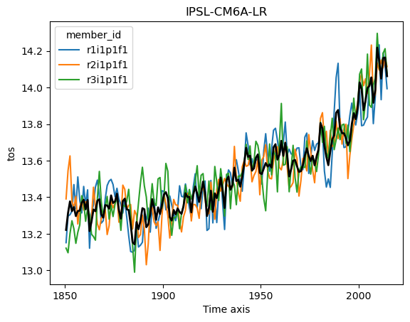
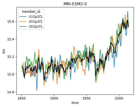
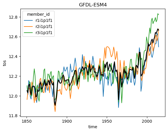
Ok but now lets analyze the data! Using what we know about xarray we can get a timeseries of the global sea surface temperature:

for name, ds in ddict.items():
    # construct yearly global mean timeseries
    mean_temp = ds.tos.mean(['x', 'y']).coarsen(time=12).mean()
    plt.figure()
    mean_temp.plot(hue='member_id')
    # lets also plot the average over all members
    mean_temp.mean('member_id').plot(color='k', linewidth=2)
    plt.title(ds.attrs['source_id']) #Extract the model name right from the dataset metadata
    plt.show()

But wait! This is not exactly right. We need to weight the spatial mean by the area of each grid cell, since the area varies based on the position on the globe (and the particularities of the curvilinear grid used in each model). But we can easily query the cell area (by modifying the query from above slightly) and then match them to the data using xmip

# Repeat the above steps to get the cell area matching the temperature we loaded earlier
cat_area = col.search(
    variable_id='areacello', # the cell area is a different variable in the collection
    table_id='Ofx', # since area is not varying in time we need to specify a different table_id
    experiment_id='historical', # Same as before
    grid_label='gn', # Same as before
    source_id=['IPSL-CM6A-LR', 'MRI-ESM2-0', 'GFDL-ESM4'], # Same as before
    member_id=['r1i1p1f1', 'r2i1p1f1', 'r3i1p1f1'], # Same as before
)
# read all datasets into a dictionary (make sure to apply the same preprocessing as before!)
ddict_area = cat_area.to_dataset_dict(
    preprocess=combined_preprocessing,
    xarray_open_kwargs={'use_cftime':True}
) 

--> The keys in the returned dictionary of datasets are constructed as follows:
	'activity_id.institution_id.source_id.experiment_id.table_id.grid_label'

100.00% [3/3 00:05<00:00]

/srv/conda/envs/notebook/lib/python3.9/site-packages/xmip/preprocessing.py:106: UserWarning: Renaming failed with 'area'
  warnings.warn(f"Renaming failed with {e}")
/srv/conda/envs/notebook/lib/python3.9/site-packages/xmip/preprocessing.py:106: UserWarning: Renaming failed with 'areacello'
  warnings.warn(f"Renaming failed with {e}")
/srv/conda/envs/notebook/lib/python3.9/site-packages/xmip/preprocessing.py:106: UserWarning: Renaming failed with 'area'
  warnings.warn(f"Renaming failed with {e}")
/srv/conda/envs/notebook/lib/python3.9/site-packages/xmip/preprocessing.py:106: UserWarning: Renaming failed with 'areacello'
  warnings.warn(f"Renaming failed with {e}")
/srv/conda/envs/notebook/lib/python3.9/site-packages/xmip/preprocessing.py:106: UserWarning: Renaming failed with 'area'
  warnings.warn(f"Renaming failed with {e}")
/srv/conda/envs/notebook/lib/python3.9/site-packages/xmip/preprocessing.py:106: UserWarning: Renaming failed with 'areacello'
  warnings.warn(f"Renaming failed with {e}")
/srv/conda/envs/notebook/lib/python3.9/site-packages/xmip/preprocessing.py:106: UserWarning: Renaming failed with 'areacello'
  warnings.warn(f"Renaming failed with {e}")
/srv/conda/envs/notebook/lib/python3.9/site-packages/xmip/preprocessing.py:106: UserWarning: Renaming failed with 'lat'
  warnings.warn(f"Renaming failed with {e}")
/srv/conda/envs/notebook/lib/python3.9/site-packages/xmip/preprocessing.py:106: UserWarning: Renaming failed with 'lon'
  warnings.warn(f"Renaming failed with {e}")
/srv/conda/envs/notebook/lib/python3.9/site-packages/xmip/preprocessing.py:106: UserWarning: Renaming failed with 'areacello'
  warnings.warn(f"Renaming failed with {e}")
/srv/conda/envs/notebook/lib/python3.9/site-packages/xmip/preprocessing.py:106: UserWarning: Renaming failed with the new name 'lon_bounds' conflicts
  warnings.warn(f"Renaming failed with {e}")
/srv/conda/envs/notebook/lib/python3.9/site-packages/xmip/preprocessing.py:106: UserWarning: Renaming failed with the new name 'lat_bounds' conflicts
  warnings.warn(f"Renaming failed with {e}")
/srv/conda/envs/notebook/lib/python3.9/site-packages/xmip/preprocessing.py:106: UserWarning: Renaming failed with 'areacello'
  warnings.warn(f"Renaming failed with {e}")
/srv/conda/envs/notebook/lib/python3.9/site-packages/xmip/preprocessing.py:106: UserWarning: Renaming failed with the new name 'lon_bounds' conflicts
  warnings.warn(f"Renaming failed with {e}")
/srv/conda/envs/notebook/lib/python3.9/site-packages/xmip/preprocessing.py:106: UserWarning: Renaming failed with the new name 'lat_bounds' conflicts
  warnings.warn(f"Renaming failed with {e}")
/srv/conda/envs/notebook/lib/python3.9/site-packages/xmip/preprocessing.py:106: UserWarning: Renaming failed with 'areacello'
  warnings.warn(f"Renaming failed with {e}")
/srv/conda/envs/notebook/lib/python3.9/site-packages/xmip/preprocessing.py:106: UserWarning: Renaming failed with the new name 'lon_bounds' conflicts
  warnings.warn(f"Renaming failed with {e}")
/srv/conda/envs/notebook/lib/python3.9/site-packages/xmip/preprocessing.py:106: UserWarning: Renaming failed with the new name 'lat_bounds' conflicts
  warnings.warn(f"Renaming failed with {e}")

list(ddict_area.keys())

['CMIP.NOAA-GFDL.GFDL-ESM4.historical.Ofx.gn',
 'CMIP.IPSL.IPSL-CM6A-LR.historical.Ofx.gn',
 'CMIP.MRI.MRI-ESM2-0.historical.Ofx.gn']

You can inspect the new dictionary ddict_area and will find that the structure is very similar to the one for surface temperature above.

ddict_w_area = match_metrics(ddict, ddict_area, 'areacello', dim_length_conflict='align')

/srv/conda/envs/notebook/lib/python3.9/site-packages/xmip/postprocessing.py:593: UserWarning: CMIP.NOAA-GFDL.GFDL-ESM4.historical.none.Omon.gn.none.tos:`metric` dimensions ['member_id:1'] do not match `ds` ['member_id:3']. Aligning the data on `inner`
  warnings.warn(msg + " Aligning the data on `inner`")

ddict_w_area['CMIP.NOAA-GFDL.GFDL-ESM4.historical.Omon.gn']

<xarray.Dataset>
Dimensions:         (x: 720, y: 576, time: 1980, member_id: 1,
                     dcpp_init_year: 1, vertex: 4, bnds: 2)
Coordinates: (12/13)
  * x               (x) float64 -299.8 -299.2 -298.8 ... 58.75 59.25 59.75
  * y               (y) float64 -77.91 -77.72 -77.54 ... 89.47 89.68 89.89
  * time            (time) object 1850-01-16 12:00:00 ... 2014-12-16 12:00:00
  * member_id       (member_id) object 'r1i1p1f1'
  * dcpp_init_year  (dcpp_init_year) float64 nan
    lat             (y, x) float32 dask.array<chunksize=(576, 720), meta=np.ndarray>
    ...              ...
    lon             (y, x) float32 dask.array<chunksize=(576, 720), meta=np.ndarray>
    lon_verticies   (y, x, vertex) float32 dask.array<chunksize=(576, 720, 4), meta=np.ndarray>
    time_bounds     (time, bnds) object dask.array<chunksize=(1980, 2), meta=np.ndarray>
    lon_bounds      (bnds, y, x) float32 dask.array<chunksize=(1, 576, 720), meta=np.ndarray>
    lat_bounds      (bnds, y, x) float32 dask.array<chunksize=(1, 576, 720), meta=np.ndarray>
    areacello       (member_id, dcpp_init_year, y, x) float32 dask.array<chunksize=(1, 1, 576, 720), meta=np.ndarray>
Dimensions without coordinates: vertex, bnds
Data variables:
    tos             (member_id, dcpp_init_year, time, y, x) float32 dask.array<chunksize=(1, 1, 64, 576, 720), meta=np.ndarray>
Attributes: (12/48)
    Conventions:                      CF-1.7 CMIP-6.0 UGRID-1.0
    activity_id:                      CMIP
    branch_method:                    standard
    branch_time_in_child:             0.0
    comment:                          <null ref>
    contact:                          gfdl.climate.model.info@noaa.gov
    ...                               ...
    intake_esm_attrs:experiment_id:   historical
    intake_esm_attrs:table_id:        Omon
    intake_esm_attrs:variable_id:     tos
    intake_esm_attrs:grid_label:      gn
    intake_esm_attrs:_data_format_:   zarr
    intake_esm_dataset_key:           CMIP.NOAA-GFDL.GFDL-ESM4.historical.Omo...

xarray.Dataset

• Dimensions:
  • x: 720
  • y: 576
  • time: 1980
  • member_id: 1
  • dcpp_init_year: 1
  • vertex: 4
  • bnds: 2
• Coordinates: (13)
  • x
    (x)
    float64
    -299.8 -299.2 ... 59.25 59.75

    cartesian_axis :

    X

    long_name :

    x coordinate of projection

    standard_name :

    projection_x_coordinate

    units :

    deg

    array([-299.75, -299.25, -298.75, ...,   58.75,   59.25,   59.75])

  • y
    (y)
    float64
    -77.91 -77.72 ... 89.68 89.89

    cartesian_axis :

    Y

    long_name :

    y coordinate of projection

    standard_name :

    projection_y_coordinate

    units :

    deg

    array([-77.907938, -77.723813, -77.539688, ...,  89.472   ,  89.6832  ,
            89.8944  ])

  • time
    (time)
    object
    1850-01-16 12:00:00 ... 2014-12-...

    axis :

    T

    bounds :

    time_bnds

    calendar_type :

    noleap

    description :

    Temporal mean

    long_name :

    time

    standard_name :

    time

    array([cftime.DatetimeNoLeap(1850, 1, 16, 12, 0, 0, 0, has_year_zero=True),
           cftime.DatetimeNoLeap(1850, 2, 15, 0, 0, 0, 0, has_year_zero=True),
           cftime.DatetimeNoLeap(1850, 3, 16, 12, 0, 0, 0, has_year_zero=True),
           ...,
           cftime.DatetimeNoLeap(2014, 10, 16, 12, 0, 0, 0, has_year_zero=True),
           cftime.DatetimeNoLeap(2014, 11, 16, 0, 0, 0, 0, has_year_zero=True),
           cftime.DatetimeNoLeap(2014, 12, 16, 12, 0, 0, 0, has_year_zero=True)],
          dtype=object)

  • member_id
    (member_id)
    object
    'r1i1p1f1'

    array(['r1i1p1f1'], dtype=object)

  • dcpp_init_year
    (dcpp_init_year)
    float64
    nan

    array([nan])

  • lat
    (y, x)
    float32
    dask.array<chunksize=(576, 720), meta=np.ndarray>

    bounds :

    lat_bnds

    cell_methods :

    y: point x: point

    long_name :

    latitude

    standard_name :

    latitude

    units :

    degrees_north

    Array Chunk Bytes 1.58 MiB 1.58 MiB Shape (576, 720) (576, 720) Count 16 Graph Layers 1 Chunks Type float32 numpy.ndarray

  • lat_verticies
    (y, x, vertex)
    float32
    dask.array<chunksize=(576, 720, 4), meta=np.ndarray>

    axis :

    Y

    long_name :

    latitude bounds

    units :

    degrees_north

    Array Chunk Bytes 6.33 MiB 6.33 MiB Shape (576, 720, 4) (576, 720, 4) Count 12 Graph Layers 1 Chunks Type float32 numpy.ndarray

  • lon
    (y, x)
    float32
    dask.array<chunksize=(576, 720), meta=np.ndarray>

    bounds :

    lon_bnds

    cell_methods :

    y: point x: point

    long_name :

    longitude

    standard_name :

    longitude

    units :

    degrees_east

    Array Chunk Bytes 1.58 MiB 1.58 MiB Shape (576, 720) (576, 720) Count 22 Graph Layers 1 Chunks Type float32 numpy.ndarray

  • lon_verticies
    (y, x, vertex)
    float32
    dask.array<chunksize=(576, 720, 4), meta=np.ndarray>

    axis :

    X

    long_name :

    longitude bounds

    units :

    degrees_east

    Array Chunk Bytes 6.33 MiB 6.33 MiB Shape (576, 720, 4) (576, 720, 4) Count 18 Graph Layers 1 Chunks Type float32 numpy.ndarray

  • time_bounds
    (time, bnds)
    object
    dask.array<chunksize=(1980, 2), meta=np.ndarray>

    long_name :

    time axis boundaries

    Array Chunk Bytes 30.94 kiB 30.94 kiB Shape (1980, 2) (1980, 2) Count 10 Graph Layers 1 Chunks Type object numpy.ndarray

  • lon_bounds
    (bnds, y, x)
    float32
    dask.array<chunksize=(1, 576, 720), meta=np.ndarray>

    Array Chunk Bytes 3.16 MiB 1.58 MiB Shape (2, 576, 720) (1, 576, 720) Count 38 Graph Layers 2 Chunks Type float32 numpy.ndarray

  • lat_bounds
    (bnds, y, x)
    float32
    dask.array<chunksize=(1, 576, 720), meta=np.ndarray>

    Array Chunk Bytes 3.16 MiB 1.58 MiB Shape (2, 576, 720) (1, 576, 720) Count 32 Graph Layers 2 Chunks Type float32 numpy.ndarray

  • areacello
    (member_id, dcpp_init_year, y, x)
    float32
    dask.array<chunksize=(1, 1, 576, 720), meta=np.ndarray>

    cell_methods :

    area: sum

    long_name :

    Grid-Cell Area

    original_name :

    areacello

    standard_name :

    cell_area

    units :

    m²

    original_key :

    CMIP.NOAA-GFDL.GFDL-ESM4.historical.Ofx.gn

    parsed_with :

    xmip/postprocessing/_parse_metric

    Array Chunk Bytes 1.58 MiB 1.58 MiB Shape (1, 1, 576, 720) (1, 1, 576, 720) Count 3 Graph Layers 1 Chunks Type float32 numpy.ndarray

• Data variables: (1)
  • tos
    (member_id, dcpp_init_year, time, y, x)
    float32
    dask.array<chunksize=(1, 1, 64, 576, 720), meta=np.ndarray>

    cell_measures :

    area: areacello

    cell_methods :

    area: mean where sea time: mean

    long_name :

    Sea Surface Temperature

    original_name :

    tos

    standard_name :

    sea_surface_temperature

    units :

    °C

    Array Chunk Bytes 3.06 GiB 101.25 MiB Shape (1, 1, 1980, 576, 720) (1, 1, 64, 576, 720) Count 14 Graph Layers 45 Chunks Type float32 numpy.ndarray

• Attributes: (48)

  Conventions :

  CF-1.7 CMIP-6.0 UGRID-1.0

  activity_id :

  CMIP

  branch_method :

  standard

  branch_time_in_child :

  0.0

  comment :

  <null ref>

  contact :

  gfdl.climate.model.info@noaa.gov

  data_specs_version :

  01.00.27

  experiment :

  all-forcing simulation of the recent past

  experiment_id :

  historical

  external_variables :

  areacello

  forcing_index :

  1

  frequency :

  mon

  grid :

  ocean data on native grid tripolar - nominal 0.5 deg latitude/longitude

  grid_label :

  gn

  initialization_index :

  1

  institution :

  National Oceanic and Atmospheric Administration, Geophysical Fluid Dynamics Laboratory, Princeton, NJ 08540, USA

  institution_id :

  NOAA-GFDL

  license :

  CMIP6 model data produced by NOAA-GFDL is licensed under a Creative Commons Attribution-ShareAlike 4.0 International License (https://creativecommons.org/licenses/). Consult https://pcmdi.llnl.gov/CMIP6/TermsOfUse for terms of use governing CMIP6 output, including citation requirements and proper acknowledgment. Further information about this data, including some limitations, can be found via the further_info_url (recorded as a global attribute in this file). The data producers and data providers make no warranty, either express or implied, including, but not limited to, warranties of merchantability and fitness for a particular purpose. All liabilities arising from the supply of the information (including any liability arising in negligence) are excluded to the fullest extent permitted by law.

  mip_era :

  CMIP6

  nominal_resolution :

  50 km

  parent_activity_id :

  CMIP

  parent_experiment_id :

  piControl

  parent_mip_era :

  CMIP6

  parent_source_id :

  GFDL-ESM4

  parent_time_units :

  days since 0001-1-1

  parent_variant_label :

  r1i1p1f1

  physics_index :

  1

  product :

  model-output

  realm :

  ocean

  references :

  see further_info_url attribute

  source_id :

  GFDL-ESM4

  source_type :

  AOGCM AER CHEM BGC

  sub_experiment :

  none

  sub_experiment_id :

  none

  table_id :

  Omon

  title :

  NOAA GFDL GFDL-ESM4 model output prepared for CMIP6 all-forcing simulation of the recent past

  variable_id :

  tos

  variant_info :

  N/A

  intake_esm_vars :

  ['tos']

  intake_esm_attrs:activity_id :

  CMIP

  intake_esm_attrs:institution_id :

  NOAA-GFDL

  intake_esm_attrs:source_id :

  GFDL-ESM4

  intake_esm_attrs:experiment_id :

  historical

  intake_esm_attrs:table_id :

  Omon

  intake_esm_attrs:variable_id :

  tos

  intake_esm_attrs:grid_label :

  gn

  intake_esm_attrs:_data_format_ :

  zarr

  intake_esm_dataset_key :

  CMIP.NOAA-GFDL.GFDL-ESM4.historical.Omon.gn

Ok the dataset now has a matching areacello coordinate that we can use to weight our results. To see the effect of area weighting we will plot both timeseries (only the member average).

plt.figure(figsize=[10, 4])
for i, (name, ds) in enumerate(ddict_w_area.items()):
    plt.subplot(1,3,i+1)
    # construct yearly global mean timeseries
    mean_temp = ds['tos'].mean(['x', 'y']).coarsen(time=12).mean()
    weights = ds.areacello.fillna(0) # ocean area can contain nans, which are not allowed for weighting
    mean_temp_weighted = ds['tos'].weighted(weights).mean(['x', 'y']).coarsen(time=12).mean()
    # lets look at the difference
    mean_temp.mean('member_id').plot(label = 'unweighted', color='r')
    mean_temp_weighted.mean('member_id').plot(label = 'weighted', color='b')
    plt.title(ds.attrs['source_id'])
    plt.legend()

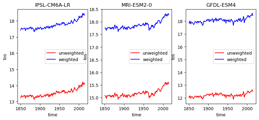
Quite the difference! This makes sense when we think about the fact that generally cells near the poles become smaller, and if we do a naive mean, these will count too strongly into the global value and reduce the resulting temperature.

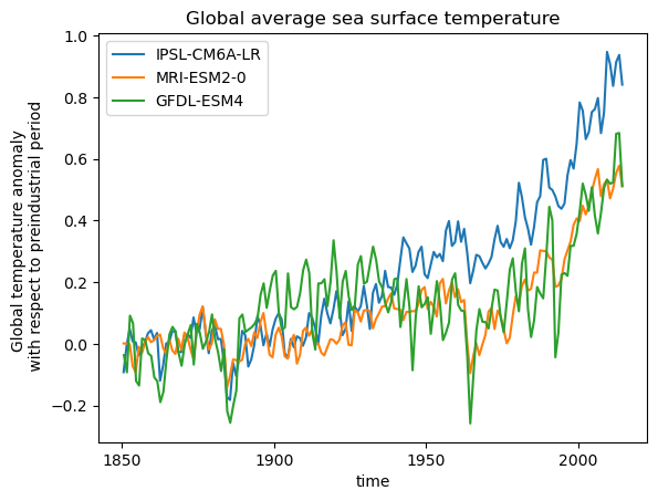
Ok lets finish by making a single nice plot of all models. In order to compare the models better we will look at the anomaly of temperature with regard to the period of 1850-1900.

plt.figure()
timeseries_dict = {}
for name, ds in ddict_w_area.items():
    # construct yearly global mean timeseries
    weights = ds.areacello.fillna(0)
    mean_temp_weighted = ds['tos'].weighted(weights).mean(['x', 'y']).coarsen(time=12).mean()
    anomaly = mean_temp_weighted - mean_temp_weighted.sel(time=slice('1850', '1900')).mean('time')
    anomaly.mean('member_id').plot(label = ds.attrs['source_id'])
plt.legend()
plt.ylabel('Global temperature anomaly \n with respect to preindustrial period')
plt.title('Global average sea surface temperature')

Text(0.5, 1.0, 'Global average sea surface temperature')

Feel free to add new models to this or maybe change the experiment, to see how each model predicts future climates.